Chapter 2 Utility Theory

Economic activity, like all other activities, is the result of a collection of individual choices. In microeconomics, we often model choices as using a utility modeling framework. Utility is the amount of ``reward’’ someone gets from some action. This reward can be in terms of wages or enjoyment. We would say that the income gained from working a part-time job bringing utility to a person but someone may gain utility from non-wage generating activities, such as being with friends, cleaning a park, or riding a bike.

Utility theory states that people have preferences over activities and people attempt to maximize their personal utility given the choices open to them. This is a relatively simple idea - we do what makes us the most happy so long as we have the time and money to do that - but it is a powerful analytic concept.

2.1 A Brief Note About Models

Economic models are used to generalize, predict, and explain behavior. They are a reduced complexity depiction of reality. It is important to note that being simple does not mean the model does not have a lot of explanatory power. As George Box, a famous statistician said in 1976: “all models are wrong, some are useful.” The power of these models is that they perform reasonably well as a way to explain why things are the way they are with minimal complexity. That is our goal. Our focus here will be on the ideas and concepts, not making highly accurate models of behavior.

2.2 Budget Sets

We assume that each individual has a budget that they are able to spend on activities that generate utility. We often think of a budget as being measured in dollars and cents, but this can be a more general concept. For instance, we must budget our time across different activities just like we budget money. We also budget our “mental wherewithal”, “spoons” in a common expression, across different tasks as well. While we will focus on budgets in terms of dollars for conceptual ease, we could just as well measure things in other units.

Suppose we have three people, each with a different budget as described in Table 2.1. All these three people care about is pizza and movies and these are the only goods they’ll spend their budget on.¹

Table 2.1: Three Hypothetical Budgets
Name	Budget
Darcy	120
Charlotte	100
Elizabeth	80

We can see that Darcy can consume up to $120/4 = 30$ pieces of pizza or $120/10 = 12$ movies, Charlotte $100/4 = 25$ pieces of pizza or $100/10 = 10$ movies, and Elizabeth $80/4 = 20$ pieces of pizza or $80/10 = 8$ movies. They could also consume any combination of pizza or movies such that they spent an amount equal to or less than their budget.

We can show the possible bundles of goods graphically, as shown in Figure 2.1.

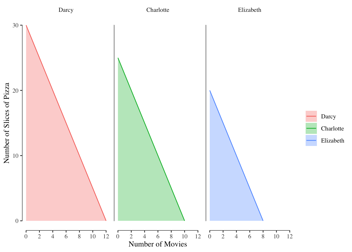
Figure 2.1: Budget Lines and Sets for Darcy, Charlotte, and Elizabeth

In each of the three panels in 2.1, the solid line shows the possible number of slices of pizza and movies consumed if the person spends their entire budget. This line is known as the budget line. In our case, where the x-axis is the number of movies and the y-axis is the number of slices of pizza, the budget line has:

x-intercept of $\frac{\text{budget}}{\text{price of movies}}$
y-intercept of $\frac{\text{budget}}{\text{price of pizza}}$
slope of $-\frac{\text{price of movies}}{\text{price of pizza}}$ or the number of additional slices of pizza you can get per movie given up

The shaded area below the budget line is known as the budget set and is the entire collection of bundles of pizza and movies that the person is able to consume with their specific budget.

An individual can consume any bundle either on the budget line or in the budget set. An individual cannot consume any bundle above the budget line as that bundle is not affordable given the current budget.

2.2.1 What About Things Without a Price?

We can also use this same framework to discuss things that do not have a direct price. For instance, leisure time does not have a price. If I check out a book from the library and sit at home reading, I am not directly spending any money. It might seem at first that these “priceless” or “price free” situations break the model. How can we use this modeling framework to understand this behavior?

While reading the library book does not have a direct cost, it does have an opportunity cost. The opportunity cost of an action is the cost created by the fact that we can only uses our resources once. If we elect to spend an hour at home reading a book, that is an hour that we cannot spend doing something else. Formally, the opportunity cost is the price of the next best thing. In the case of staying at home and reading, a leisure activity, we assume the next best use of the time is to work and earn money.

Suppose if instead of staying home and reading, we could work a shift at work and earn an extra $10/hour. In that case by electing not to work, we are, in effect, spending $10/hour due to forgone income. This opportunity cost, the $10/hour we’d earn if working, is the cost of the leisure time.

The concept pf opportunity costs enables use to translate everything into dollars and cents, which we do for simplicity.

2.3 Utility Functions

The main idea of utility theory is that each person have a utility function, we’ll call it $U()$, that allows us to estimate the utility that person derives from their activities and spending.

Let’s make that a little more concrete. Suppose people derive joy only from two sources: pizza and movies. Nothing else makes them crack even the slightest smile. Pizza costs $4 per slice and movies cost $10 per showing.

2.3.1 Preferences

Different people are, well, different. Some people may strongly prefer pizza to movies while others may not care for pizza. We describe these differences between people as preferences, which allows us to incorporate difference levels of “liking” for different goods.

Let’s return to our three hypothetical people and add some preferences for them. Charlotte really likes going to see movies relative to pizza, Darcy likes both about the same, and Elizabeth prefers pizza to movies. Each of the three people, their budget, and good preference are re-capped in Table 2.2.

Table 2.2: Three Hypothetical Budgets with Preferences
Person	Budget	Favorite Good
Darcy	120	Equal
Charlotte	100	Pizza
Elizabeth	80	Movies

This means that Charlotte will require a greater number of movies to give up a slice of pizza then Darcy or Elizabeth as she places a greater value on pizza than on movies. Likewise, Elizabeth will want a greater number of slices of pizza to give up a movie than Darcy or Elizabeth. Additionally, for a given budget, the optimal bundle will contain the most movies with Elizabeth and the least with Charlotte and the most pizza with Charlotte and the least with Elizabeth. These imbalances in the number of goods in each bundle is the result of the differences in preferences between the different people.

2.3.2 Indifference Curves

Much of utility theory relies on comparing the utility of different bundles for a person. Suppose a bundle $A$ has 3 movies and 3 slices of pizza and we want to compare that against a bundle $B$ with 4 movies and 2 slices of pizza. Plausible changes in utility² for each of three people at bundles $A$ and $B$ are shown in Table 2.3.

Table 2.3: Comparison of Utility at Two Bundles
Names	Utility at 3 pizza, 3 movies	Utility at 2 pizza, 4 movies	Change in Utility
Elizabeth	3.8	4.2	0.4
Darcy	2.2	2.1	-0.1
Charlotte	3.8	3.1	-0.7

We see that Elizabeth is much happier with bundle $B$ compared to bundle $A$ as her utility increased by 0.4 units. Elizabeth prefers A to B or $A \prec B$³ Meanwhile both Darcy and Charlotte are less happy with $B$ than $A$ as their utility decreased. We write this as Darcy and Charlotte $A \succ B$. Because Charlotte prefers pizza even more than Darcy, her decrease in utility from $A$ to $B$ is even larger.

One particularly informative question is “how many more slices of pizza would it take for you to be equally happy with one fewer movie?” This concept of “equally happy” is known formally as indifferent. A person is indifferent between two bundles of different compositions if they are equally happy with either bundle. We denote indifference between two bundles as $A \sim B$.

For instance, let’s suppose everyone currently has 3 slices of pizza and tickets to 3 movies. How many slices would pizza would be required to be equally happy with only 2 movies? Likewise, how many movies would be required to be equally happy with 2 slices of pizza?

Table 2.4: Change in Pizza and Movies to be Indifferent
name	Movies at 2 Pizza	Pizza at 2 Movies
Elizabeth	3.5	8.3
Darcy	4.5	4.5
Charlotte	8.3	3.5

We see that Elizabeth, who strongly prefers movies to pizza, requires an 8.3 slices of pizza, or 5.3 more, to give up a single movie while she would be willing to give up a slice of pizza in exchange for only 0.5 more movies. Darcy, who likes both pizza and movies equally, is willing to give up 1 for 1.5 more of the other. Charlotte, in a mirror of Elizabeth, requires 5.3 more movies to give up a single slice of pizza and is only willing to give up half a slice for an additional movie.

The idea of indifference between bundles leads us to draw indifference curves. Indifference curves are a line, which is generally curving, on which every combination of goods has equal utility for the person. These curves help us understand how people approach the tradeoff of giving up or gaining an additional unit of a particular type of good.

For example, we can draw the line describing all combinations of bundles that give Darcy, Elizabeth, and Charlotte exactly 2 utility points, shown in Figure 2.2.

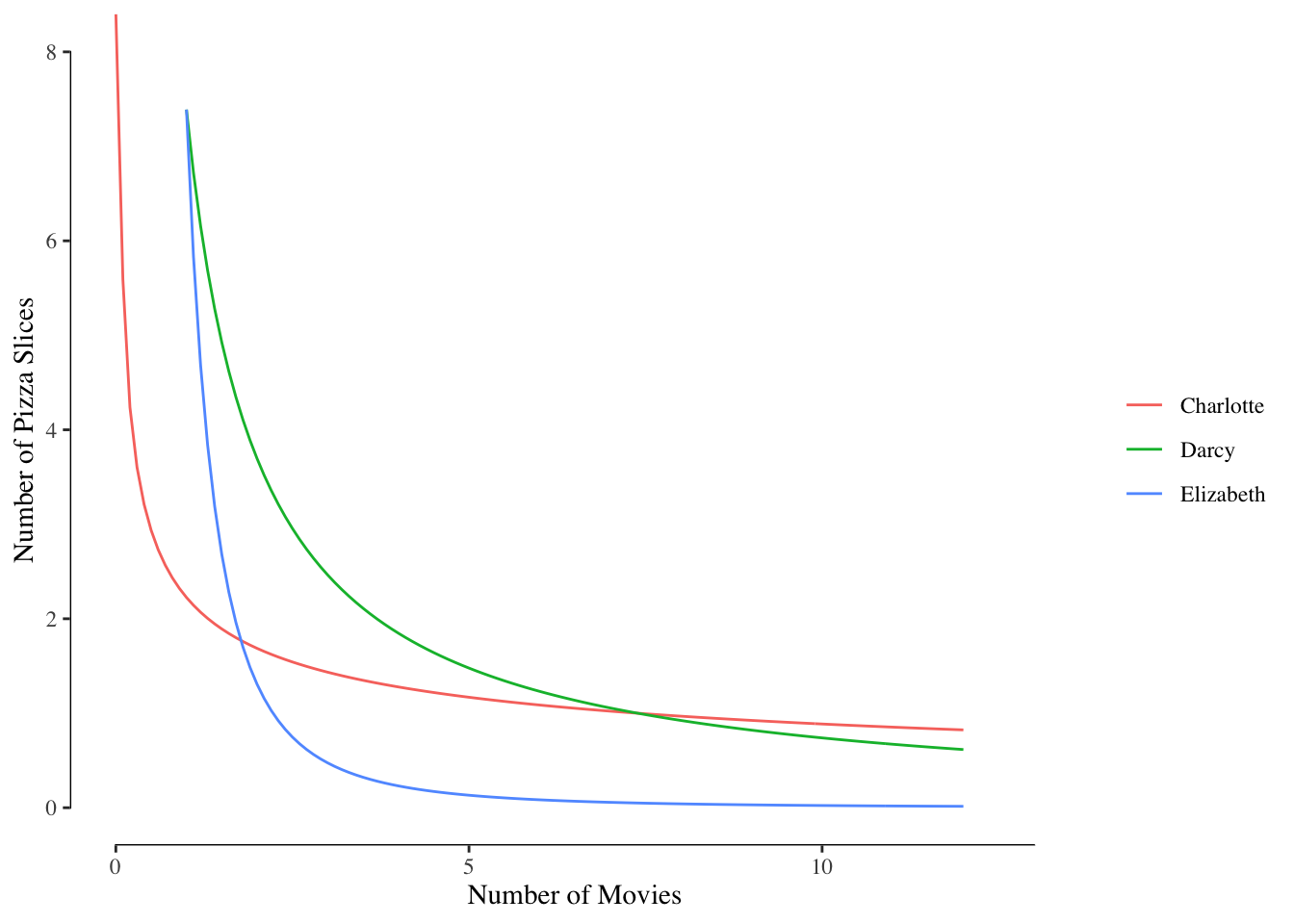
Figure 2.2: Indifference Curves at 2 Utility

We see that Charlotte’s curve is almost flat - she requires many movies to give up a small amount of pizza. This is the result of her preference for pizza. Elizabeth’s curve is very steep - she requires many slices of pizza to give up a small amount of movies. Darcy’s curve, with his middling preference for both pizza and movies, is more balanced between the two.

2.3.3 Marginal Utility

In economics, we are often interested in decision making at the margin. This simply means we are interested in how things change by adding one more of something to a pile you already have. We are interested in the value of the next slice of pizza for someone who has 10 slices and how that compares to the value for someone who has only 1. This value of the next slice is pizza is called the marginal utility.

Notice that the indifference lines in 2.2 are not flat straight lines but instead curve. This is the result of a concept called diminishing marginal utility. In short, the marginal utility of something decreases the more of that you have.

The concept is intuitive: the more of something you have, the less you value more of it. Someone with 10 slices of pizza would not value the 11th slice of pizza as much as someone getting the first slice of pizza. Same with movies: the fourth movie you see in a week isn’t as valued as the first movie you see.

Graphically, this causes the indifference curves to flatten out as you move to higher numbers of one type of good. This is most clear on Darcy’s curves. If you follow along an axis, you’ll notice that with each additional movie Darcy sees, he becomes less willing to give up pizza for an additional movie (in other words, he gives up less pizza per additional movie). Likewise, when Darcy has many slices of pizza, he becomes less willing to give up movies (he gives up fewer movies per additional slice of pizza). As Darcy has more of a single type of good, the marginal utility of one more decreases.

We can describe the marginal utility at different points by comparing the utility, given a person’s preferences, at $(\text{number of movies}, \text{number of pizza slices})$ to $(\text{number of movies} + 1, \text{number of pizza slices})$ for the marginal utility of movies or $(\text{number of movies}, \text{number of pizza slices} + 1)$ for the marginal utility of pizza.⁴

The marginal utility for both pizza and numbers is shown in Figure @ref(fig:marginal_utility). We see that Charlotte, who prefers pizza, always has higher marginal utility of pizza than she does of movies. Likewise, her marginal utility of pizza is always higher than either Darcy’s or Elizabeth’s. Elizabeth is the opposite with higher marginal utilities of movies than pizza. Darcy’s marginal utility of movies and pizza is the same in this case because of how the utility function was expressed but this won’t always be the case.

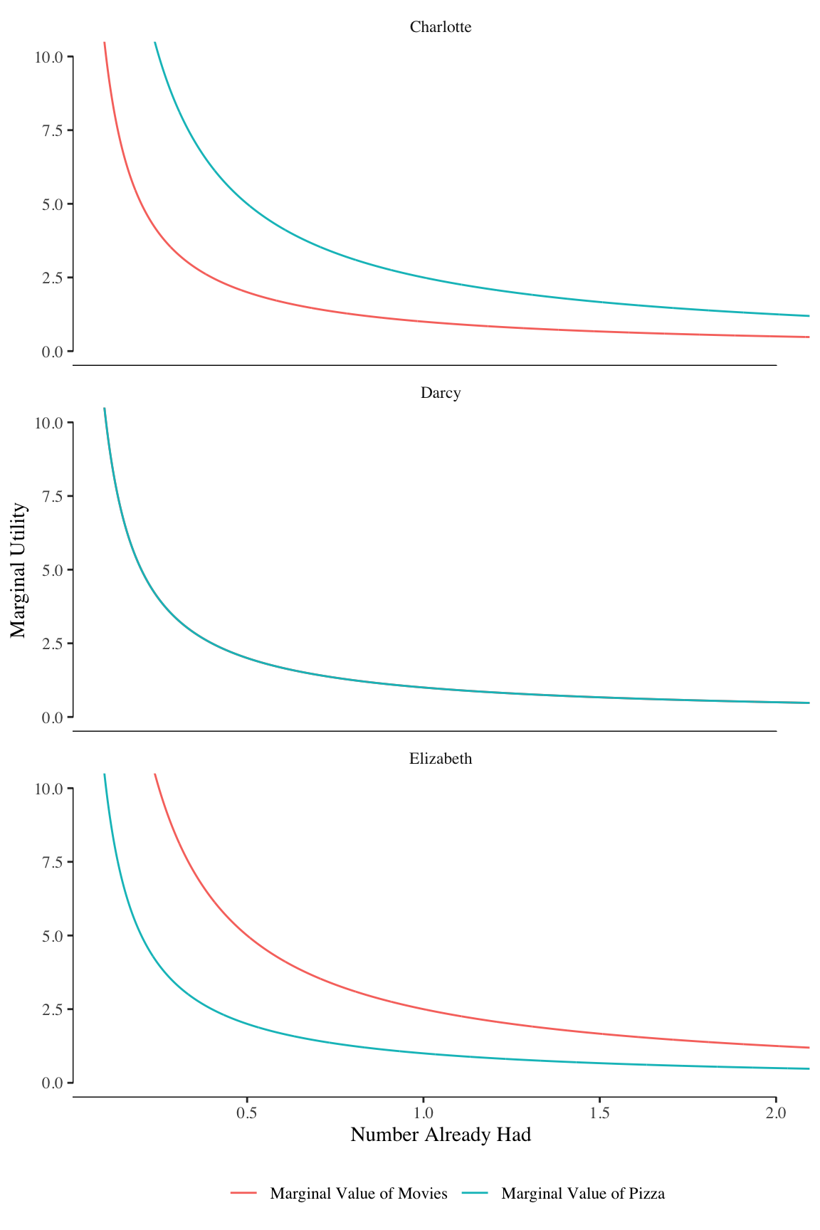
All three people exhibit the diminishing marginal utility expected. For each additional unit of movies or pizza that they consume, the increase in utility they get goes down.

2.3.4 Marginal Rate of Substitution

We extend this concept to the marginal rate of substitution (MRS). The marginal utility (MU) expressed the increase in utility that the person got from gaining one additional unit of goods. The marginal rate of substitution describes a similar idea: what is the number of items of a good that I’d be willing to trade away, or substitute, for one more item of the second good while remaining indifferent between the two bundles?

In more concrete terms, let’s assume the current bundle is $(m = 3, p = 3)$. The question asked by MU is how much more utility would I gain from moving to $(m = 4, p = 3)$, the marginal utility of movies, or $(m = 3, p = 4)$, the marginal utility of pizza. The MRS is instead focused on the value of the “$?$” when moving from $(m = 3, p = 3)$ to $(m = 4, p = ?)$ or $(m = ?, p = 4)$ if the utility of the basket does not change.

We can find this value by moving along an indifference curve. Figure 2.3 shows the MRS for moving from the bundle containing 2 movies (located at $A$) to a new bundle with 3 movies at $B$.

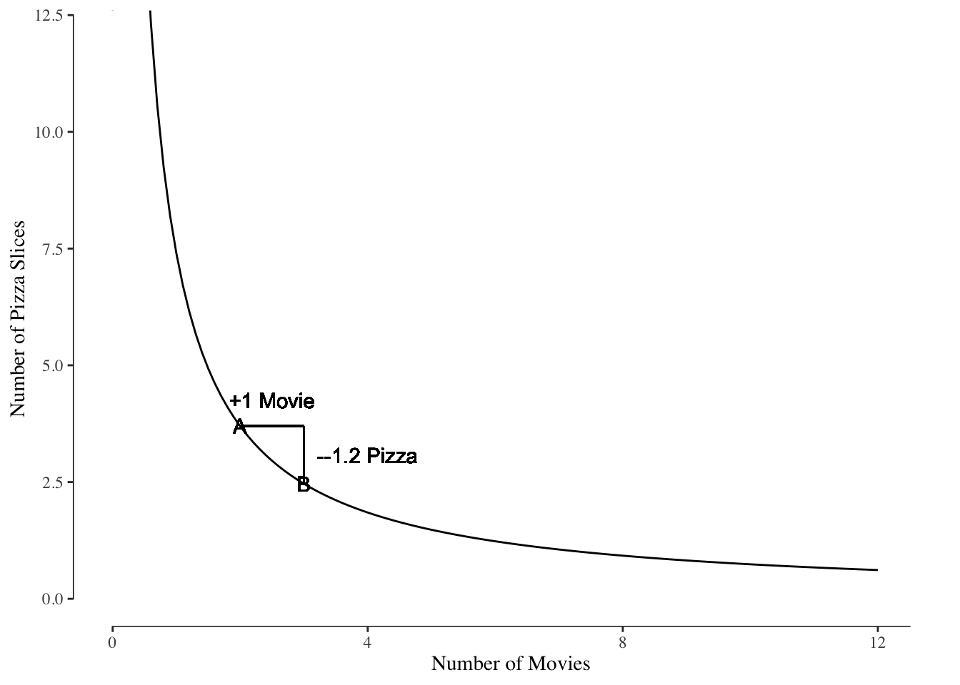
Figure 2.3: MRS Example

Darcy, the source of this indifference curve, is indifferent between a bundle with 2 movies and about 3 slices of pizza and one with 3 movies but 1.2 fewer slices of pizza. In other words, Darcy will give up 1.2 slices of pizza for 1 movie if he has, at present, 2 movies.

Notice that the MRS changes with the number of movies or pizza in the current bundle. Figure 2.4 shows the same indifference curve as Figure 2.3 $C$ but the starting bundle contains 5 movies instead of 2. At a bundle with 2 movies, Darcy is willing to trade 1.2 slices of pizza for an additional movie; however, starting with 5 movies, he is only willing to trade 0.2 slices for an additional movie.

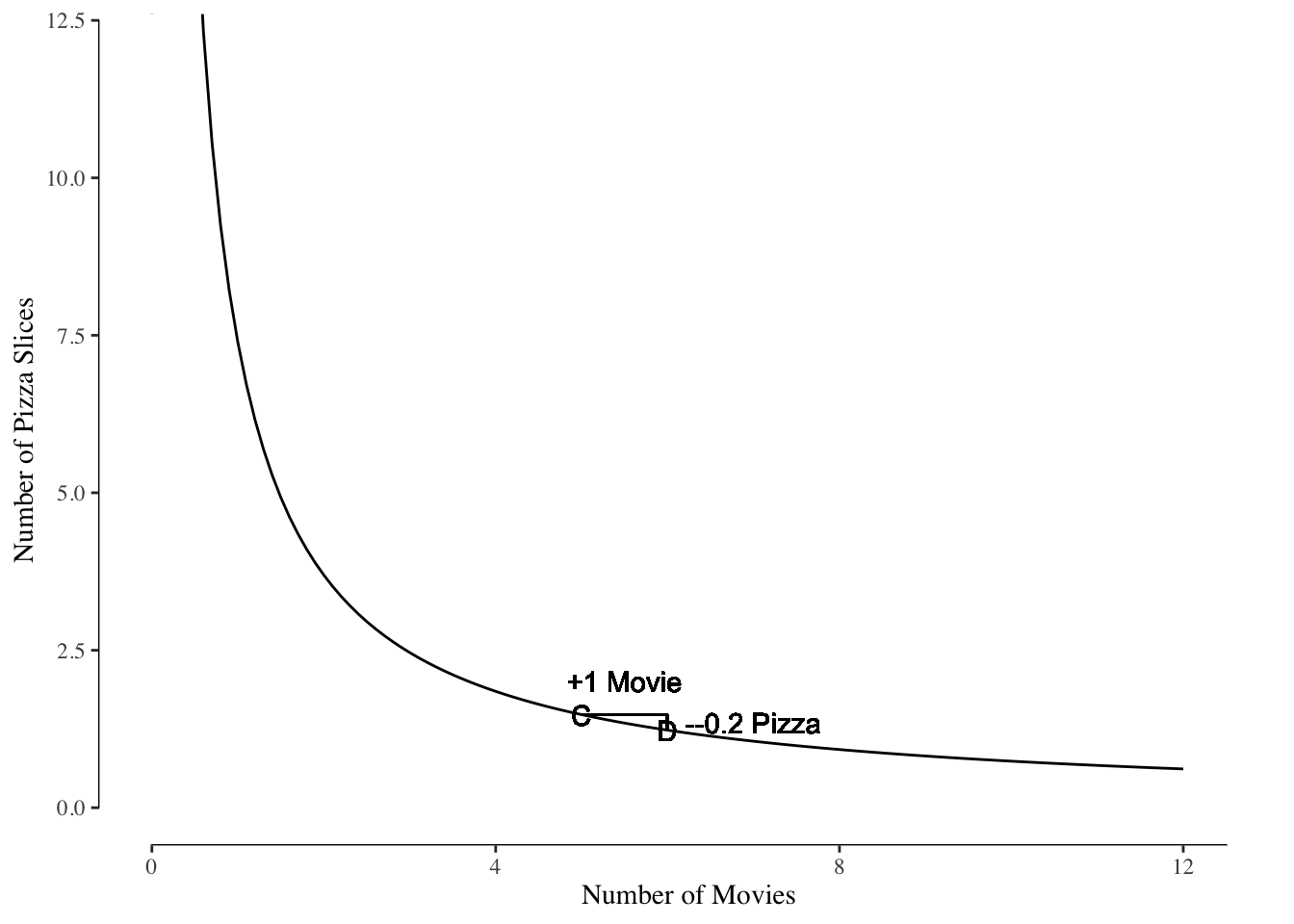
Figure 2.4: MRS Example at Large Bundle Sizes

This makes sense intuitively: The more of something we have, the less we value it relative to other goods. Thinking the situations shown in Figures 2.3 and 2.4. Bundle $A$ contains fewer movies than bundle $C$ and so the marginal movie, bundled $B$ and $D$ has greater value at bundle $A$ than $C$. This greater marginal utility of the movies at $B$ than $A$ compared to $D$ than $C$ means that a greater number of slices of pizza must be given up for to remain indifferent between the bundles.

Recalling from earlier, the slope of the budget line was

\[\text{slope of budget line} = -\frac{\text{price of good on x-axis}}{\text{price of good on y-axis}}\]

reflecting the relative prices of the two goods. The price of the good is constant - we pay the same price for the 9th item as the 3rd item - and so the ratio is just the prices for all the different combinations of movies and pizza.

Likewise, the slope of the indifference curve is the ratio of the marginal value of each good. Price reflected the marginal cost to acquire an additional unit and the marginal value reflects the marginal increase in utility to acquire an additional unit. Following from the example of the slope of the budget line, we see then that the slope of the indifference curve at bundle $(m, p)$ is

\[\text{slope of indifference curve} = - \frac{\text{MU}_m(m, p)}{\text{MU}_p(m, p)}\]

or the ratio of the marginal utilities at the current bundle.⁵

2.3.5 More is More

Would you rather have 3 slices of pizza or 2 slices of pizza, all else equal?

Three slices, right? If you are hungry, 3 slices is better than 2 slices and, even if you aren’t hungry right now, having extra slices in the fridge is better than having no left over pizza. If you are offered a free slice of pizza, you take it.

In economics, this is known as non-satiation, or the idea that more is always better. A bundle with 3 movies and 3 pizzas is always worse than a bundle with 4 movies and 3 pizzas, even if you don’t like movies much.

Graphically, this concept results in utility curves moving to the right. Three indifference curves at utilities of 1, 1.75, and 2.5 are shown in Figure 2.5. As the utility increases, the location of the curve shifts to the right. Indifference curves more to the right are at higher levels of utility than curves more to the left.

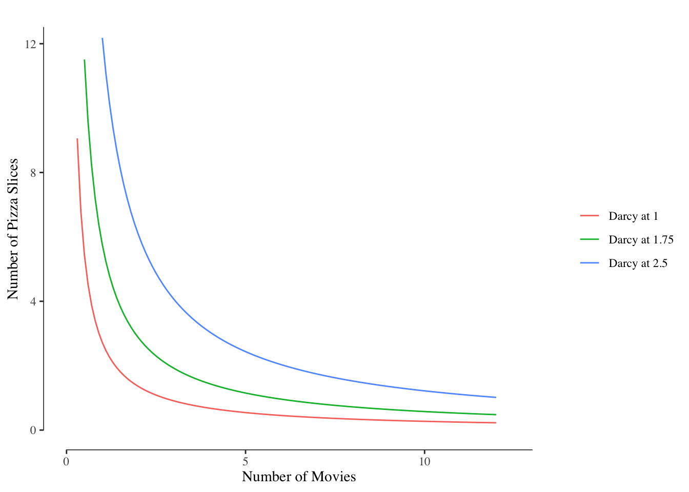
Figure 2.5: Indifference Curves for Darcy at Different Utility Levels

2.4 Where is the Best Bundle

We know from Figure 2.1 that the consumed bundle must be on or below the budget line in order to be in the budget set.

We know from Figure 2.5 that a bundle located on an indifference curve further to the right is preferred to a bundle located on an indifference curve located to the left.

These two statements give us the exact location of the optimal bundle. The optimal bundle occurs where the budget line is intersected, but not crossed, or tangent to an indifference curve. Why?

2.4.1 The Bundle Must Be On The Budget Line

It is simple to show that the bundle must be on the budget line through the principle of non-satiation. Let’s consider Darcy’s budget set shown in Figure 2.6.

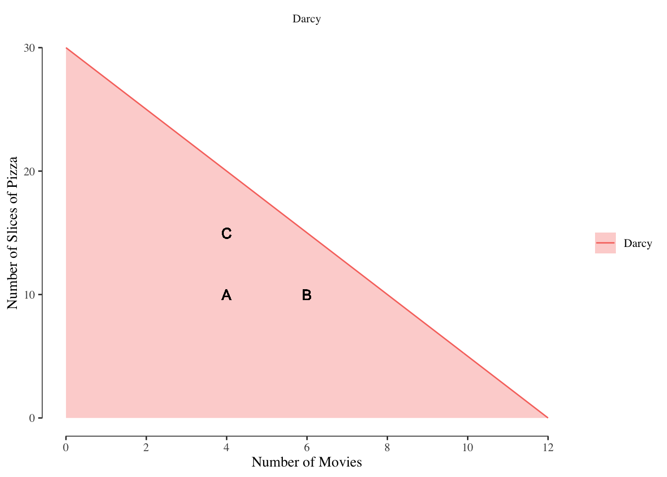
Figure 2.6: Consumption Options in Darcy’s Budget Set

Suppose Darcy is consuming bundle $A$ which has 4 movies and 10 pizzas. It is also within his budget to consume 6 movies and 10 pizzas, shown as bundle $B$, or to consume 15 pizzas and 4 movies, shown as $C$. Since $B$ has the same number of slices of pizza but more movies then $A$ we have $B \succ A$. Likewise, since $C$ has move pizza but the same number of movies as $A$, we have $C \succ A$. Since all $A$, $B$, and $C$ are affordable bundles, we know the optimal bundle cannot be $A$.

Let’s shift the location of bundle $A$ such that the bundle is on the budget line. We’ll call this new bundle $A'$. Now if we add more movies at $B'$ or more pizza at $C'$, we find ourselves outside of the budget set. While either $B'$ or $C'$ would preferable to $A'$, they are not affordable because they fall above the budget line. This is shown in Figure 2.7.

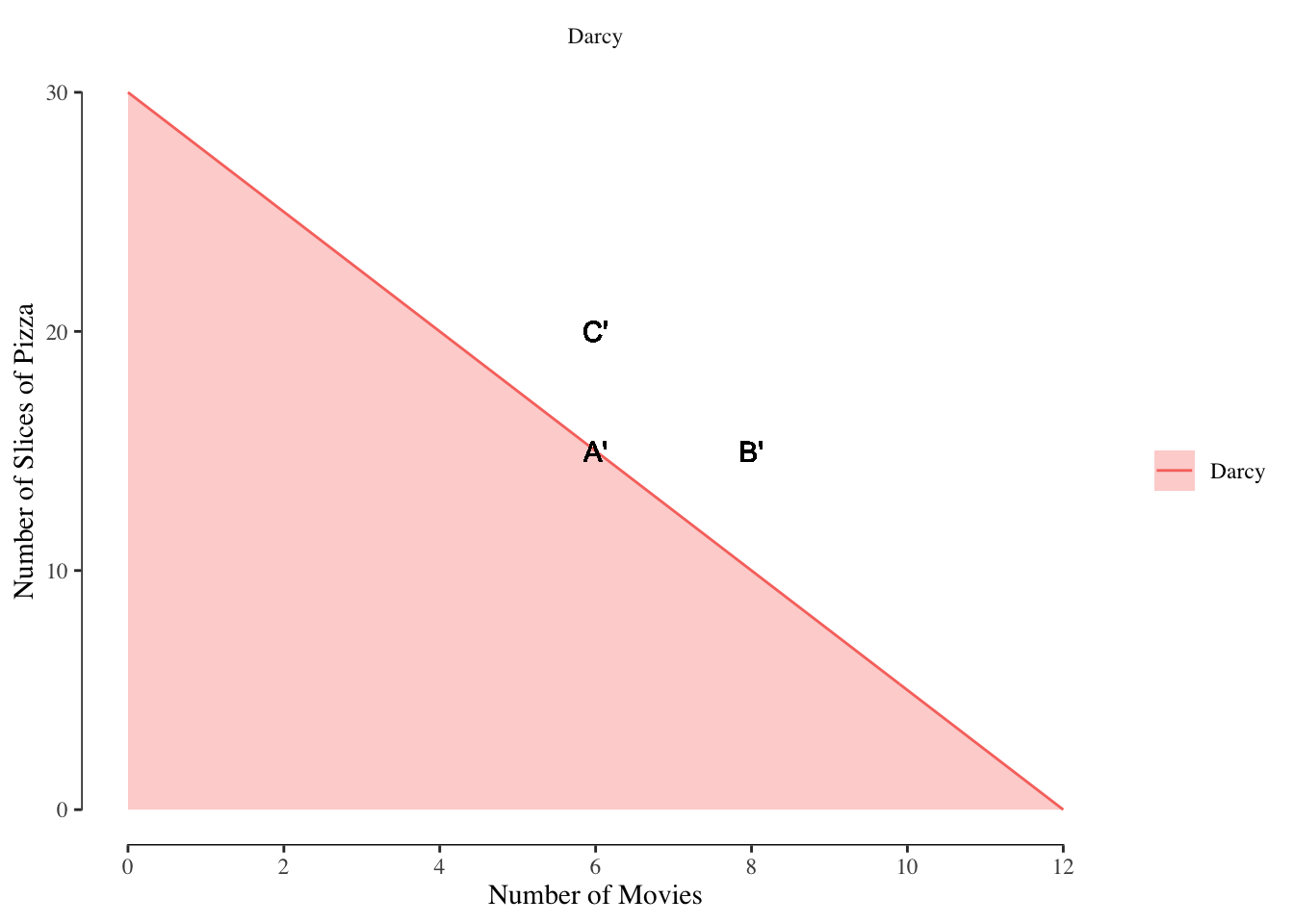
Figure 2.7: Consumption Options on the Budget Line

2.4.2 The Bundle Must Be Where The Budget Line is Tangent to an Indifference Curve

Now that we know the optimal bundle must be on the budget line, the next step is determining which point on the budget line is optimal. The optimal bundle occurs at point where the budget line is tangent to an indifference curve.

A line is tangent to a curve if they intersect but only at one place. Three possible indifference curves and the budget set for Darcy are shown in Figure 2.8.

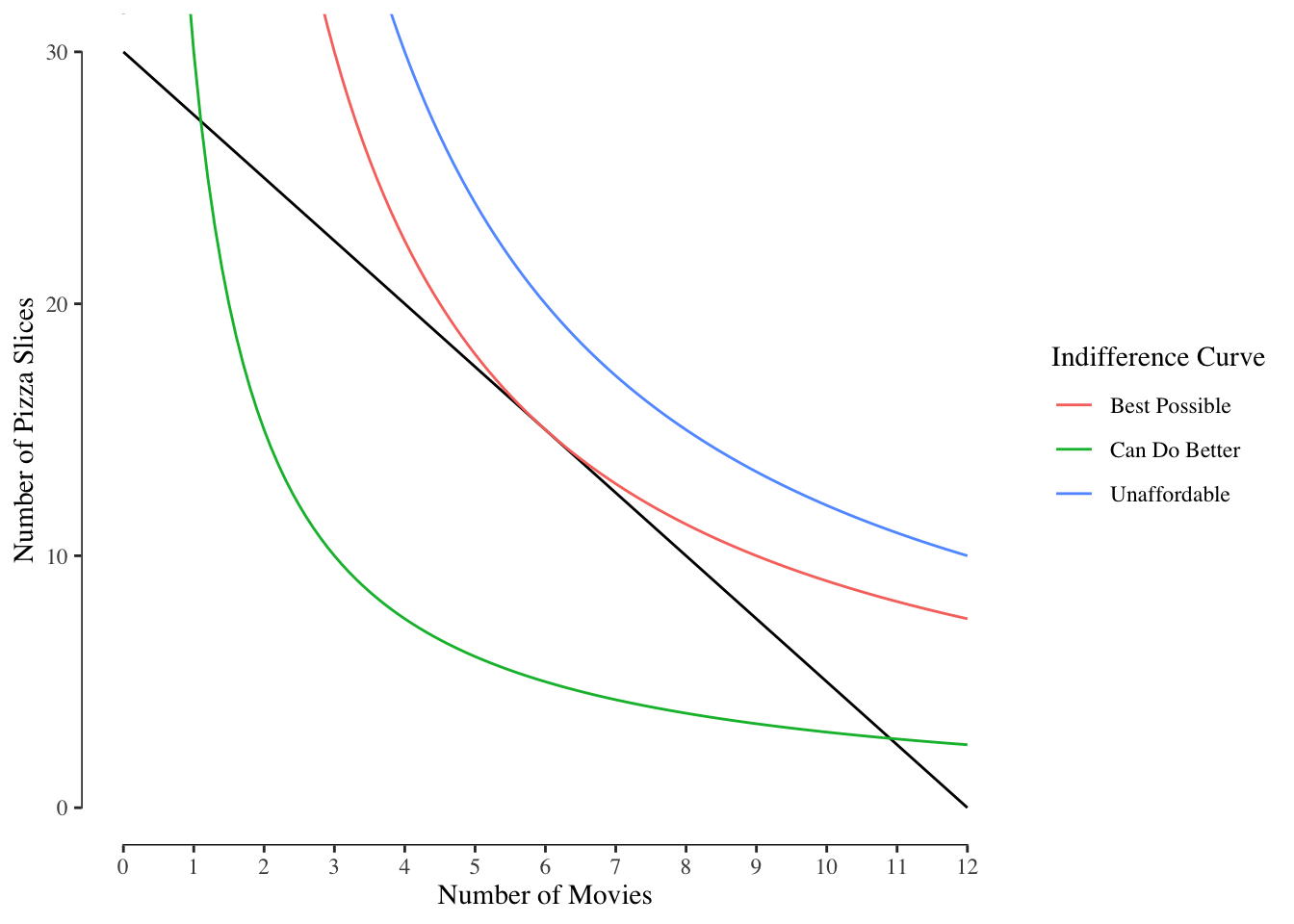
Figure 2.8: Three Indifference Curves and Budget for Darcy

Of the three curves, only one is optimal.

The line labeled “Can Do Better” is not optimal because it contains points in the budget set and not on the budget line. Bundles in the budget set but not on the budget line cannot be the best bundles, as shown in 2.6. Since the bundles at the intersection of the budget line and the indifference curve provide the same utility for Darcy as those inside the budget set, we know a better bundle is possible.
The line labeled “Unaffordable” does provide the highest utility but since it does not intersect with the budget line or enter the budget set, there are no combinations on that indifference curve that can be purchased with our budget.
The line labeled “Best Possible” is the indifference curve that is tangent to the budget set. This means that the indifference curve intersects the budget line at exactly one point. There is only one bundle on the budget line that is on the indifference curve and there are no points inside the interior of the budget set. No curve further to the right, in other words with more utility, can be drawn while still intersecting the budget line.

Due to the different budgets and different preferences, everyone will have different optimal bundles. The optimal bundles for our three hypothetical people shown in Figure 2.9. The dashed lines denote the budget line for each of the three people, the solid lines are the optimal indifference curves, and the dot denotes the location of the optimal bundle.

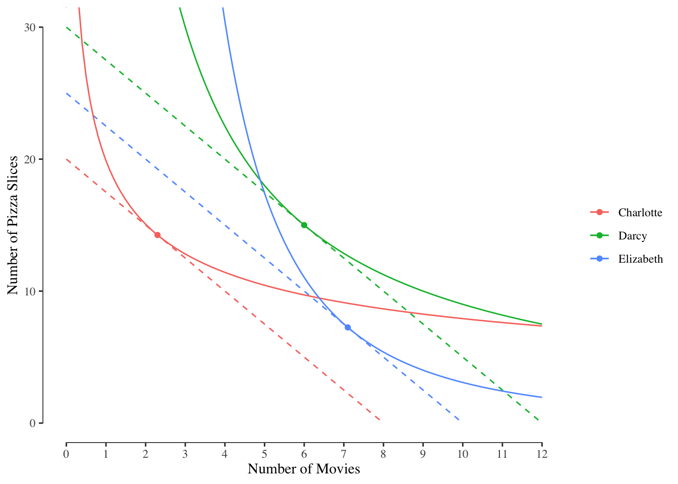
Figure 2.9: Optimal bundles for all three example people

Due to the differences in budgets, each person spends a different total amount of money on movies and pizza. However, the distribution changes between the people. Darcy spends half his money on movies and half on pizza, but Charlotte, who prefers pizza, spends 71% of her budget on pizza while Elizabeth spends 71% on movies. This reflects differences in their consumption habits.

2.5 Utility Theory and Public Health

Utility theory is often a theoretical tool used to motivate models to describe why people behave the way they do. Many models are used in public health and you may be familiar with some such as social cognitive theory, theory of planned behavior, or the health belief model, all of which are similar in intention to utility theory. The goal of these models is to understand behavior.

We could model, for instance, someone’s decision to smoke tobacco. We would suppose they have two goods: smoking tobacco and health. They can increase their tobacco consumption at the cost of having less health or increase their health consumption at the cost of smoking less tobacco. We will suppose that “health” here includes all future health as the immediate effects of smoking tobacco are likely small.⁶ We suppose that some people may have greater preferences for health and opt not to smoke while others may have lower preferences for health or greater preferences for the “pleasure” of smoking leading them to make different decisions.

This same framework can be used to understand other lifestyle habits such as diet or exercise with little modification. We could also use utility theory to understand why some people get vaccinated, wear masks during the COVID-19 pandemic, or take other health protective measures.

Utility theory, in general, is somewhat more encompassing and broad than the frameworks developed out of non-economics social sciences. Ultimately, at the end of the day, all of these frameworks provide a theoretical basis for understanding why people make the choices they make.

In our example, we assume only two goods brought people joy: pizza and movies. Is certainly doesn’t reflect the real world as people enjoy a lot of things beyond pizza and movies. Is this example model too simple, too silly to be of value in the real world?

Perhaps surprisingly, no. The simple two good model is incredibly powerful for describing real world decision making. Everyone likes pizza (even those who dislike pizza “like” pizza, just with “zero” weight) and they also like other things. We could simply replace “movies” with “all goods that aren’t pizza” and the same graph can be made. In this case, we changed a particular good of movies to become a composite good of “all goods that aren’t pizza.”

Likewise, we could use this graph to describe the process someone undergoes when deciding how many hours to work. We could label one side of the graph as “hours spent working”, or more directly “wages”, and the other side as “leisure.” The number of leisure activities is uncountable but that is okay for our purposes.

The key to these simple budget sets and utility models is that they are highlighting a tradeoff. We like to think of the tradeoff between two specific things (e.g., pizza and movies) but we could just as easily use a composite good on one axis.↩︎
Here we assume that the utility is given by $U = p_m \text{log}(m) + p_p \text{log}(p)$ where $p_m$ and $p_p$ are the preferences for movies and pizza, respectively, and $m$ and $p$ are the number of movies and pizza consumed. We use the $\text{log}$ transformation to create a series of curves with diminishing marginal utility, which is discussed in later sections. We assume $p_m$ and $p_m$ are $(2.5, 1)$ for Elizabeth, $(1, 1)$ for Darcy, and $(1, 2.5)$ for Charlotte. These numbers and the function are totally made up as conceptual representations.↩︎
Why the weird symbols? We could write $U(A) < U(B)$ as we are comparing the utility of the different bundles but that is a bit of a hassle with all the extra $U$’s to write. Since $A$ and $B$ refer to a bundle of goods or a set, it isn’t technically correct to write $A < B$. Instead, we use the “curved” versions of of the greater than/less than signs to denote which bundle or set is preferred as a sort of shorthand.↩︎
This is also the slope of the line with respect to the good that we are changing. You may recall from calculus that this would be the first derivative of the utility function with respect to the good that is changing.

Our utility function is $U = p_m \text{log}(m) + p_p \text{log}(p)$. Based on this, our marginal utility of pizza is
\[\frac{\partial U}{\partial p} = \frac{p_p}{p}\]
and the marginal utility of movies is
\[\frac{\partial U}{\partial m} = \frac{p_m}{m}\]
A graphical understanding is good enough for this course but if you have the math background the calculus-based explanation may be helpful. If it is, use it. If it isn’t, ignore it.↩︎
For our hypothetical utility function, the MRS is \[MRS = -\frac{\text{MU}_m(B)}{\text{MU}_p(B)} =-\frac{p_m / m}{p_p / p}\]
Since utility is constant on an indifference curve, we can rewrite $p$ in terms of utility $U$ and $m$:
\[\text{MRS} = -\frac{p_m / m}{p_p / \exp\bigg(\frac{U - p_m \log(m)}{p_p}\bigg)}\]
Which, after cross-multiplication, becomes:
\[\text{MRS} = -\frac{p_m \exp\bigg(\frac{U - p_m \log(m)}{p_p}\bigg)}{p_p m}\]
We can arrive at the same result through calculus. First, we re-write the utility function as an indifference curve:
\[p = \exp\bigg(\frac{U - p_m \log(m)}{p_p}\bigg)\]
Then, we take the partial derivative with respect to $m$:
\[\frac{\partial p}{\partial m} \exp\bigg(\frac{U - p_m \log(m)}{p_p}\bigg)= -\frac{p_m \exp(\frac{U - p_m \log(m)}{p_p})}{p_p m}\]
which gives us the same value as above.↩︎
We will get into the detailed weeds of modeling some choices that lead to harm later in the course, especially using a concept called “rational addiction.” Additionally, future effects of our courses require some additional consideration that we omit here but discuss later.↩︎