Chapter 7 Empirical Methods
So far we’ve acted as though we know the effect of an externality exactly but have not considered how we estimate the effect of an externality. In this chapter, we consider empirical methods. This chapter is not going to be a complete description of empirical methods in public health or policy research, you have other classes to cover those ideas in detail (e.g., biostatistics or epidemiology classes) but instead will focus on the why we do empirical research, issues we face while doing empirical work, and two methods that are used with increasing frequency to study public health questions.
7.1 Causality
In general, in public policy, we are interested in what causes the outcomes that we want to change and not what merely is correlated with or predicts the outcomes. We are interested in things that are causally related to the outcome - things that cause the outcome. This is important because our focus is often on policy changes and changing a factor correlated with, but not causally related to, our outcome will fail to have the desired effect.
Consider this somewhat obvious example: there is a strong relationship between ice cream sales and drowning deaths, shown in Figure 7.1.
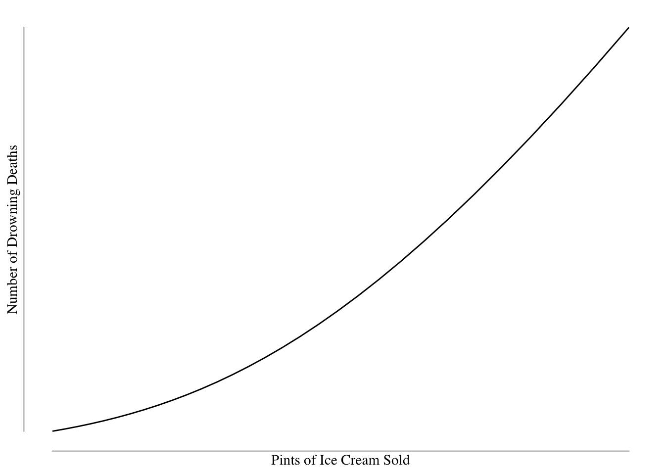
Figure 7.1: Relationship Between Quantity of Ice Cream Sold and Number of Drowning Deaths.
Based on this graph, it would seem that consumption of ice cream leads to an increased risk of drowning. We might want to regulate ice cream to prevent the deaths - perhaps ban selling ice cream on the beach or at the pool to prevent drowning.
However, such a policy would almost certainly fail to change the number of drowning deaths. It is unlikely that ice cream causes drowning - it is much more likely that a variable we’ve ignored causes both ice cream sales and encourages swimming. Such a variable might be temperature. Temperature causes both an increase in swimming (and therefore drownings) and an increase in demand for ice cream, Figure 7.2.
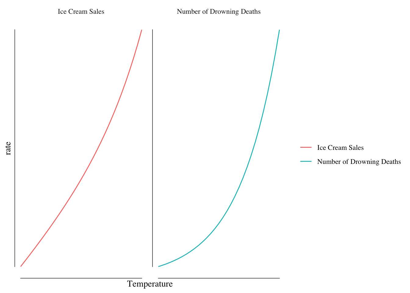
Figure 7.2: Relationship Between Ice Cream Sales/Drowning Deaths and Temperature.
Once we account for the relationship between temperature and both drowning and ice cream sales, we find no effect of ice cream sales on drowning rates.
While ice cream sales were correlated with our outcome of drowning, they did not cause drowning and so policy changes focused on ice cream could not have the effect we desire. It is critical when designing policy to push levers that are causally related to our outcomes.
However, outside of simple examples, determining what causes something can be quite challenging. We often struggle with issues of confounding and bias in our studies. For instance, we may find that frequently attending a casino is associated with lung cancer. However, people who frequent casinos may be more likely to smoke and casinos often allow smoking, increasing the exposure to second-hand smoke even among non-smokers. It is not gambling in this case that may increase cancer risk but rather behaviors and exposures associated with gambling. We would say the relationship between gambling and lung cancer is confounded by smoking rates.
Bias is another example where we can get estimates that are misleading. The insurance company Geico advertises that “drivers who switch save 15% or more on their car insurance.” This number is likely true but does not mean that if you call you are likely to save 15%. The only people who switch their insurance are those people that are offered a better rate by Geico then their current insurance company. As a result, the typical savings will not be the same as the savings reported by drivers who switched. Mentally, we conflate the average savings offered with the average savings of those who saved.
This process of building our sample can introduce bias into our result and cause us to not estimate the number that we want to know. While Geico quotes the “drivers who switched” number because that is better advertising, when doing policy work that would not be the number we are interested in. Care needs to be taken when building our sample to make sure we are collecting the right data on the right people and not introducing bias into our analysis.
The gold standard for dealing with these problems is a randomized controlled trial. In such a trial, we recruit a relatively large number of people and assign them to a treatment/exposure/policy that we are interested in or assign them to not have that treatment/exposure/policy. Since the assignment is random any differences between the two groups will balance out and allow us to make an estimation of the effect of the treatment/exposure/policy.
Suppose we were interested in the rate at which people experience head injuries and have a new protocol for preventing damage from these injuries. We recruit student-athletes for our sample and take baseline measurements and randomize them to either using the new cognitive-protection tool or to usual care. The risk of head injury is not the same across all of our student-athletes: football players will have higher risk than cross-country runners, gymnasts will have higher rates than rowers, and so on. However, since these people are randomly assigned to the two groups, the average rate in the two groups will be the same. As a result, we can ignore the fact that football players are at greater risk than runners and focus on the differences between the groups.
However, there are limitations with randomized controlled trials, both comically highlighted by papers in the British Medical Journal. Ever December, the British Medical Journal publishes a light-hearted research article. In 2003, they published a paper titled “Parachute use to prevent death and major trauma related to gravitational challenge: systematic review of randomised controlled trials” by Gordon Smith and Jill Pell. The paper looked at randomized trials of parachutes to prevent death or injury when falling from an airplane and found no trials had been done. The reason why no trials had been reported is obvious: throwing a person from an airplane without a parachute would not be ethical.
Many questions that we are interested would not be ethical to study with a randomized controlled trial. I might be interested in whether smoking is actually protective against neurodegenerative diseases like Parkinson’s disease, something we frequently see in large data samples, but it would not be ethical to randomly force people to smoke. I might be interested in if a certain drug is safe in pregnancy or if it causes birth defects, but I could not randomly assign women to take the medication. We often have questions where the answer cannot be arrived at using a randomized trial for ethical reasons.
The second paper, published in the British Medical Journal in 2018 is a reply to the review by Smith and Pell. Yeh and others performed a randomized controlled trial of parachutes to prevent injury or death when jumping from an airplane. They reported their results in a paper titled “Parachute use to prevent death and major trauma when jumping from aircraft: randomized controlled trial.” They gave half the participants parachutes and half empty backpacks to determine if the parachute prevented injury when they jumped from the airplane. They found that parachutes did not reduce the rate of injury or death compared to backpacks and, furthermore, the rate of injury with backpacks was 0. What is omitted from their title was that the aircraft were parked and on the ground when the participants jumped with a mean altitude of a few feet.
While this was obviously in jest, it is a real problem with randomized controlled trials. Consider the HPV vaccine trial. HPV is a very common virus transmitted between humans through sexual contact. The virus can cause cancer and so preventing infection will prevent cancer. When designing this trial, you would not want to recruit anyone who likely already had the virus (80% of sexually active adults), so you would want to recruit people who are likely not to have yet been sexually active. You also would not want to recruit people who are unlikely to be sexually active during the study period. The trial was mostly interested in preventing cervical cancer in women, so you would not want to recruit any men in the trial. Finally, you would want to recruit people who are normally healthy and likely to respond to the vaccination. The trial found the vaccine worked to prevent infection, cancer, and was safe. But that trial tells us nothing about how effective the vaccine would be in
- Men of any age
- Women who are sexually active or older but do not have HPV infection
- Women who are younger than the trial cohort
- Women who have weaker than normal immune systems or other pre-existing conditions
As a result, the vaccine was initially only approved for women of a relatively narrow age range.
Other trials are similar - we don’t include very old or very sick people in trials of drugs like statins. These people are unlikely to be informative in a clinical trial and will create noise, making the trial harder to do. However, when we go into the real world, we have older, sicker people. The groups recruited in the trials will be balanced and the estimate will be valid for those groups; however, whether that estimate is applicable to the population at large is uncertain.
The reason for these exclusions is that randomized trials are expensive to conduct. There are significant logistical and cost barriers to large trials. Trials that require long duration of follow-up are often prohibitively expensive. For these reasons, we often use observational research methods.
7.2 Observational Research
Most policy research is observational - we observe the changes that occur in the real world. This differs from the randomized trials in that exposures, treatments, or policies are not assigned at random or by the researcher. For instance, mask mandates and “shelter-in-place” orders appear to reduce the spread of COVID-19. However, these policy changes were applied for some reason not selected by the researcher and this can create problems.
Suppose that mask mandates are issued, as they were in Iowa City, in anticipation of a surge in the number of cases following the return of the University to the classroom and the reopening of the bars in downtown Iowa City. The reason for the mandate was related to the outcome (e.g., we expected cases to increase) and therefore if we simply compared the incidence rate in Iowa City to Cedar Rapids before and after the mask mandate, we would not get an accurate estimate of the effect of a mask mandate on spread.
A more common concern is that the mask mandate or “shelter-in-place” order is issued when things are getting bad or at their peak. These orders are a reaction to the current status. However, when things are “really bad” there is, in generally, only one way out: for them to get better. Incidence typically would fall over the next month even if the orders were completely non-effective. This would make mask mandates or shelter-in-place orders look more effective than they truly are.
Almost none of our choices are done “at random” and the concern is that if our choice is related to factors that affect the outcome, then we need to be careful in how we estimate the effect of that choice.
Public health uses two primary types of study designs when looking at the effect of a policy or exposure.
The first is a cohort study. A cohort study identifies people with the exposure or subjected to the policy of interest and a second group of people without that exposure. We then compare the rate of outcomes (e.g., disease) between the two groups. For example, if we were interested in the effect of fracking on the rate of low-birthweight babies, we could identify a group of babies born to parents who lived near fracking sites and a second group of babies that were born to parents who did not live near fracking sites. We would then compare the rates of low-birthweight between the two groups.
The second major design is a case-control study. In a case-control study, we identify people who have the outcome of interest (our cases) and a second group who does not (out controls). We then compare the odds of disease given exposure between the two groups. For example, we may be interested in the relationship between lung cancer and smoking. We identify people who have lung cancer and a second group of people of similar age without lung cancer and then determine who did and did not smoke. We then compare the odds of disease between smokers and non-smokers using an odds ratio.
In practice, we use matching (e.g., if we have a male case, we want a male control) and regression to “adjust for” these confounders. This has been a very brief overview of these methods as you’ve likely seen them before. We want to focus on two methods that are likely more novel for public health undergraduate students: differences-in-differences and regression discontinuity.
7.3 Difference-in-Differences
Differences-in-differences, commonly called diff-in-diff, is a method for comparing pre/post policy changes using a control group. For instance, we may identify a city or state where some policy or event occurs and find the difference between our outcome measure after and before the event. Let’s call this \(\Delta Y_{I}\) for the change in the outcome \(Y\) in the intervention location.
This is the change we observed with the policy change; however, other trends may be occurring that we need to control for using a control group. These control observations are the change in the outcome in places similar to the intervention location but that did not have the policy go into effect. We estimate this difference and call it \(\Delta Y_{C}\).
The value \(\Delta Y_{C}\) gives us an idea of what we would have expected the change to be in the intervention area if they had not use the policy or had the event. So the effect of the policy, \(\Delta P = \Delta Y_I - \Delta Y_C\). This is how the method gets it’s name, it is the difference between the differences before and after the policy in the intervention and control locations.
It can be helpful to consider an example. Differences-in-differences has been most famously used to study the effects of increasing the minimum wage. Card and Krueger are two economists who used difference-in-differences to study this question. Standard economic theory would suggest raising the minimum wage would decrease the quantity of labor demanded by employers who pay minimum wage. Card and Krueger tested this idea by looking at fast food restaurants (who pay minimum wage for many employees) in New Jersey and Pennsylvania before and after New Jersey, but not Pennsylvania, increased the minimum wage in 1992.
The law went into effect in April of 1992 and the study compared the average hours worked per restaurant in February and November of 1992. They found the typical New Jersey restaurant had 20.44 FTEs (one FTE = 40 hours) in February while one in Pennsylvania had 21.03 FTEs. After the law went into effect, the number of FTEs increased, on average, to 21.03 in New Jersey and decreased to 21.17 in Pennsylvania. In other words, from February to November, the typical restaurant in New Jersey increased their FTEs by 0.59 while one in Pennsylvania decreased by 2.16. Based on these results, Card and Krueger estimated the effect of increasing the minimum wage to be an increase of 2.75 FTE per restaurant.
The inclusion of a “control group,” in our example the restaurants in Pennsylvania, is a key advantage of difference-in-differences. Suppose between our first measurement and our post-policy measurement something major had happened - a pandemic, a general economic slowdown, a large influx of money - that changed the environment we were operating in. For instance, suppose we were studying the effect of a tax on alcohol served in restaurants and our “before” measurement was January 2020 and and our after was October 2020. If we did not account for the pandemic depressing the number of people going to restaurants (and therefore depressing the number of people buying alcohol in restaurants), our estimates would not be meaningful. By having a control group subject to largely the same economic and other forces, we are protected against that problem.
Difference-in-differences is widely used to study policy changes (e.g., taxes, restrictions of medication) that occur on a city, county, or state basis. For instance, we could use a design to study the effect of the mask mandate in Iowa City. The mandate was issued on July 21st, 2020. We can compare the total number of new cases during the 21 day period before and after the mask mandate was issued in Johnson and Linn Counties.
| County | 21 Days Before | 21 Days After | Difference | Per 100k |
|---|---|---|---|---|
| Johnson | 517 | 482 | -35 | -22.5 |
| Linn | 409 | 824 | +415 | +183 |
Johnson and Linn Counties are similar in many respects (similar economic forces, similar populations) but differed after the mask mandate in the sense that Iowa City had one while Linn County didn’t. We saw the three weeks after the mandate that Iowa City had an incidence rate 22.5 per 100,000 lower than the three weeks before while Linn County saw an increase of 183 per 100,000 during the same time period. Putting these together, we would conclude that Johnson County’s rate was about 200 cases per 100,000 over those three weeks lower than we would have otherwise expected.
When doing a difference-in-differences analysis, you want to ensure that your control locations are valid comparison locations for the analysis. In the examples, I used Linn County as a comparison for Johnson County and the minimum wage study used an adjoining state. These are reasonably plausible comparisons. We would not want to compare, say, a rural county in Iowa to Johnson County or New Jersey to Montana. The quality of our inference depends on our control group having a parallel trend to our policy-treated group. If this assumption is violated, we may not have accurate estimates.
7.4 Regression Discontinuity
Regression discontinuity is a complicated name but a simply idea. One of the most straightforward applications is in studying the effect of being accepted to a highly selective university (say Harvard or MIT) over going to a less selective (and much less expensive) university (we’ll call it Nevada Bob’s School of Miseducation).
One problem we will immediately face is that students who attend Harvard or MIT are different than those who attend Nevada Bob’s School of Miseducation. They may have higher test scores, greater levels of focus and determination, and greater levels of family resources/networks. If we simply compare the average income of graduates of MIT to Nevada Bob’s, we’ll find a difference but it is unclear if the difference is due to attending MIT.
One way to avoid this is to look at the waitlist. Every college has a waitlist of students who are “accepted, if there is space.” Every year some number of students are admitted off the waitlist. Let’s suppose MIT has a waitlist of 200 students and they are ranked 1 to 200 and admitted in that order (e.g., the first student on the waitlist is accepted before the second). Of the 200 students, 50 are admitted to MIT. Let’s narrow our focus to those students with waitlist ranks of about 50. Is there a real difference between the students ranked 46, 47, 48, 49, and 50 versus those ranked 51, 52, 53, 54, and 55? Probably not - the students who just barely didn’t get off the waitlist are likely similar to the students who just barely got off the waitlist.
However, because students ranked 46 to 50 were accepted and students ranked 51 to 55 were not accepted there is a difference - whether they went to MIT or elsewhere. We can compare what happens to the students just barely accepted to the students just barely not accepted to estimate the effect of being accepted. Since they are otherwise quite similar, we should be able to get a good estimate of the effect. We look for a jump, or discontinuity, in their income at the rank where the last person was taken off the waitlist. Figure 7.3 shows some simulated data.
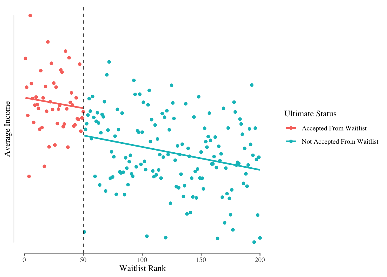
Figure 7.3: Income by Rank on Waitlist and Acceptance Status.
We can see a relationship between waitlist rank and income with higher ranks having lower incomes. We also see a “jump” in income at the point where the last student was taken off the waitlist. That jump is our estimated treatment effect.
Regression discontinuity is a powerful design whenever you have a continuous exposure that is converted into levels. For instance, the health risks of having an A1C, a measure of blood sugar, just below the threshold for treatment is likely similar to having an A1C just above the threshold. Our bodies are biological systems that do not react to somewhat arbitrary divisions. We may be interested in determining the effect of being diagnosed with diabetes on health as when someone is diagnosed, they are often treated. The same approach could be used to study the effect of being diagnosed with high blood pressure with the idea that those with borderline blood pressure, whether normal or high, are likely similar to each other.