Chapter 10 Political Economy
Government’s rarely make decisions based exclusively on cost-benefit analysis and guidance from policy experts and economists. We see this time and again in poverty assistance programs in the United States.
It would likely be better for people experiencing poverty to simply give them money and let them decide how best to use the money for their needs. As with markets, we assume people know what is best for them, individually, and are better judges of what they need than another person. While there are certainly violations of this idea - a topic we’ll return to when we discuss behavioral economics - it is a reasonable assumption unless we have evidence to the contrary. Cash transfers would enable the person to make the best decisions for themselves given their current situation and needs.
Instead, TNAF, one of the federal welfare programs, provides small payments (up to $500 for a family of 4 per month) to families below the federal poverty line comes with many strings attached. In Kansas, as an example, beneficiaries are prohibited from spending the money on tattoos, movies, getting their nails done, lingerie, or cruises.29
Other programs, like SNAP, commonly called food stamps, have restrictions on the items that can be purchased. For instance, SNAP cannot be used to purchase hot foods or foods intended for immediate consumption.30 You can buy a take-and-bake pizza from Hy-Vee with EBT but you cannot buy a cooked pizza from Hy-Vee. In 2017, the federal government was considering restricting SNAP dollars from being used to buy soda and other beverages.31
There are frequent calls for drug testing people who get SNAP, TNAF, or other government provided assistant with many states requiring a drug test before people can be on these programs.32
Little of this makes sense, economically. The way in which SNAP and TANF beneficiaries spend their money is a lot like how most people spend their money: on shelter and food, rarely on “silly” things.33 Restrictions add costs to these programs but it is unclear that the costs actually create any value. States that require drug testing almost certainly spend more on the drug testing then they would have spent on assistance that went to people who failed the drug tests.34
Given that these programs are not as effective as a form of public policy as simply giving people cash would be, it stands to reason to ask “why do we do it this way?” There is an expression that “data don’t drive” - data can guide our decision making but ultimately what decisions we make are political. The economic study of why governments make the choices they do is called political economy and is the subject of this chapter.
We’ll start with some idealized examples that are informative but unrealistic before moving to discussions of more complicated and plausible models of government behavior. In particular, we’ll focus on the median voter theorem and Arrow’s impossibility theorem for understanding the choices our governments make.
Once we’ve established an understanding of how governments make decisions, we’ll focus on times when the median voter theorem likely does not apply. In particular, we will focus on the effects of gerrymandering, voter concentration, and political polarization.
10.1 Lindhal Pricing
The Swedish economist Erik Lindahl developed a model for determining the extent to which a government should fund public goods. This approach, first described in 1919, says the government should survey individuals about their marginal willingness to pay for a public good. The marginal willingness to pay for something is the same as our demand for something: the demand curve simply tells us how much more we’d pay for another item. If we could known the marginal willingness to pay for each person, we could aggregate these demand curves to determine the societal willingness to pay. This is exactly the process we used in the public goods chapter to build the societal demand for a public good.
The process proposed by Lindahl was straight forward:
- We offer a range of tax prices for a public good
- Each person tells us how much of the good they’d want at each price
- We add the quantity demanded at each price over all the people
- We determine where this aggregate demand curve and the marginal cost curve intersect
- We tax people according to their personal willingness to pay for that quantity.
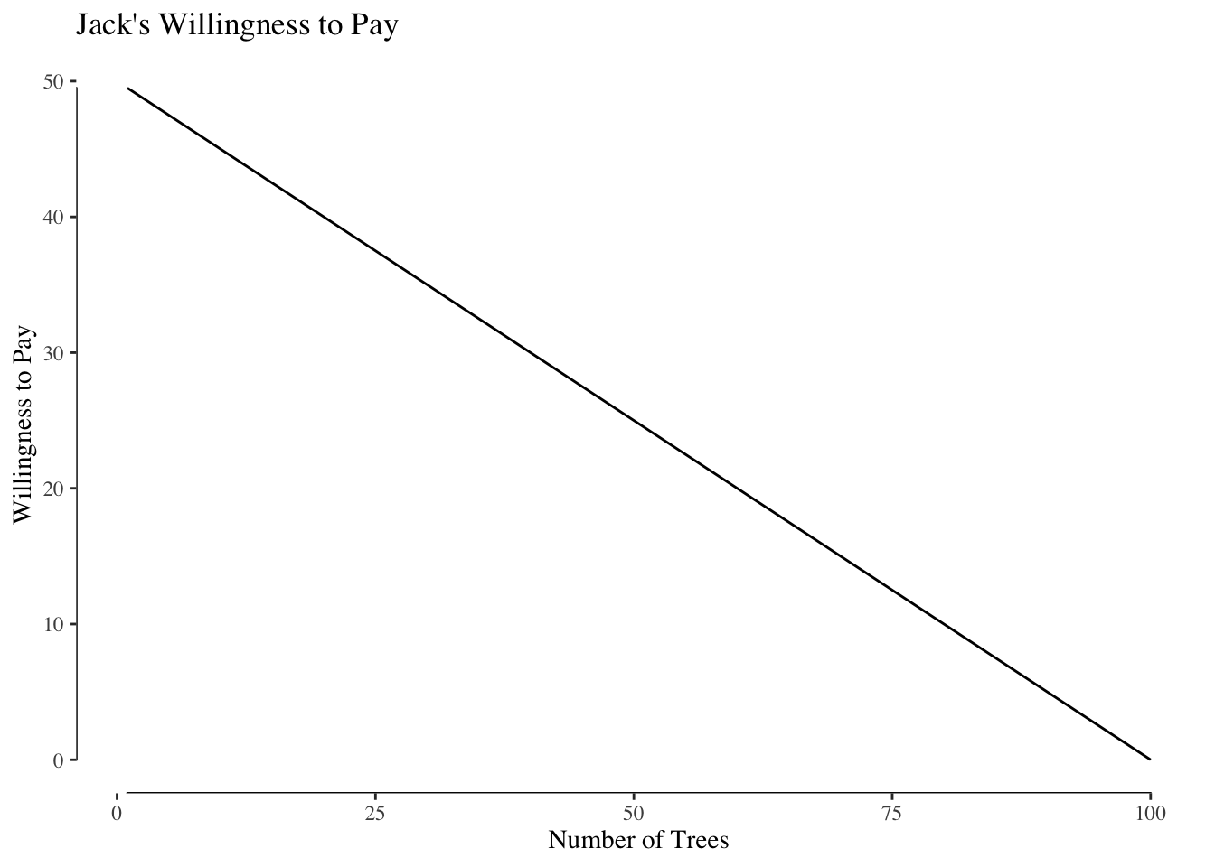
More concretely, suppose we have two consumers in our market: Jack and Nicole. Our market is for planting shade trees along the streets near where they live. The shade trees are non-rival (the number of people seeing the trees does not reduce their value and the number of people using the shade relative to the total capacity is small) and non-excludable (they provide shade along the public sidewalk) and are therefore public goods. Jack and Nicole must agree on the level of street trees.
Suppose Jack puts relatively little value on these trees. He doesn’t mind the sun and so the shade trees provide somewhat low value. Jack values the trees according to the curve shown in Figure ??.
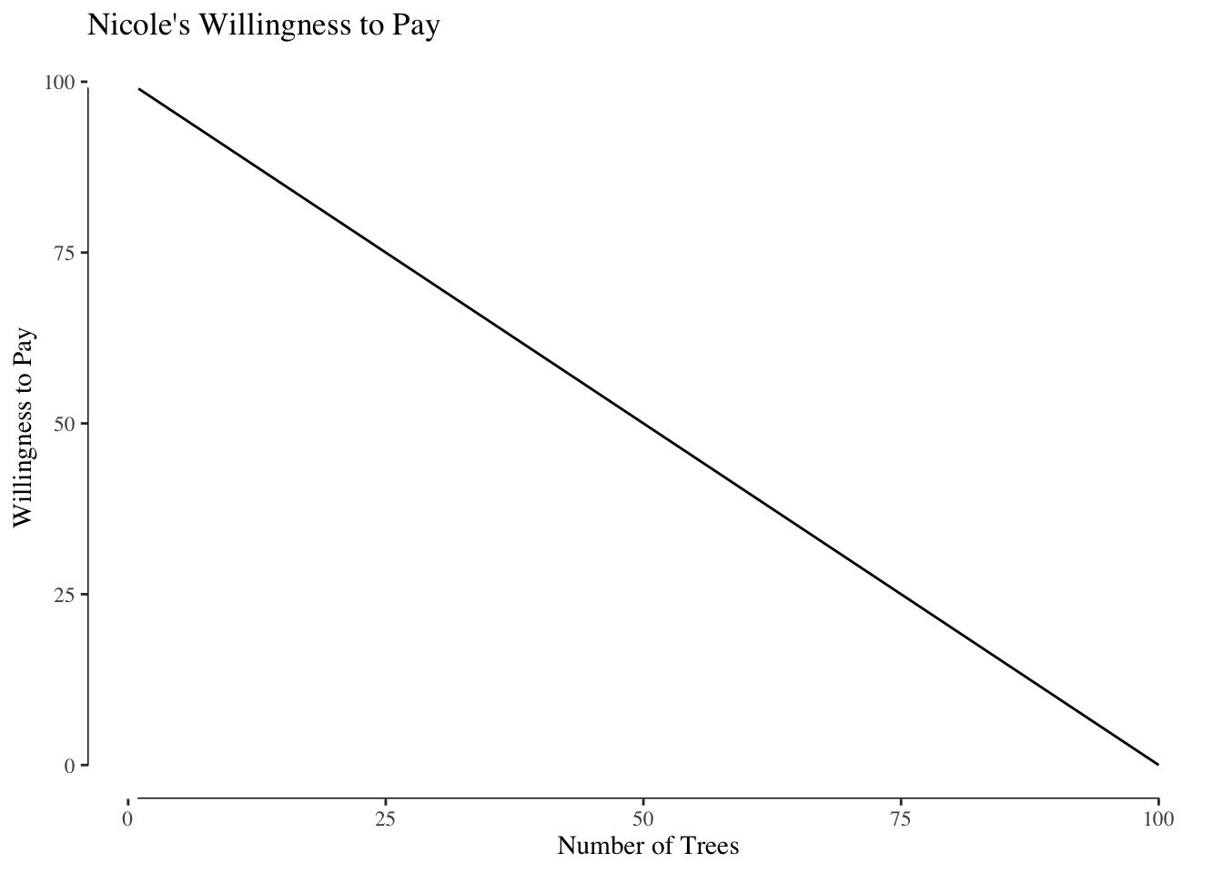
On the other hand, Nicole values trees much more than Jack. She gets sunburns easily and so wants more shade. Her demand is shown in Figure ??.
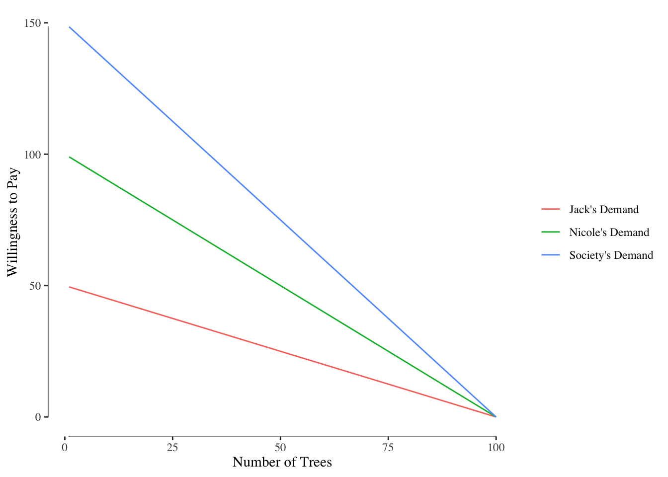
To get society’s total willingness to pay or society’s demand, we sum these two curves vertically, Figure ??.
Let’s suppose each tree costs the city a flat $30 to buy. We can add that to our market, Figure ??, and determine that the socially optimal level of street trees is to plant 80 street trees (the point where the marginal cost equals to the societal demand).
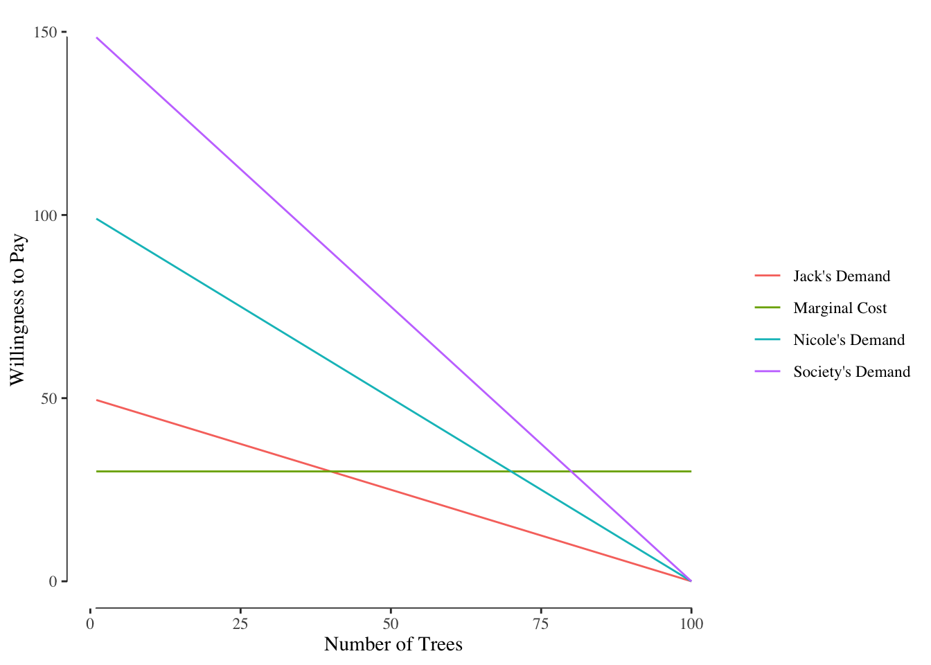
To determine how much to charge Jack and Nicole to pay for these shade trees, we look at their individual demand curves at the socially optimal quantity. We see at 80 trees that Nicole’s marginal willingness to pay is $20 while Jack’s marginal willingness to pay at 80 trees is $10. We then levy a tax of $10 on Jack and $20 on Nicole for each tree we plant.
We end up at this point for two reasons. The first is that Nicole and Jack are happy to pay those prices for the number of trees provided. Since their total willingness to pay matches the marginal cost, the government is also happy to provide that number of trees.
There are some nice features of Lindahl pricing. The different tax values on the Jack and Nicole is and example of benefit taxation because the tax amount is related to the person’s valuation of the benefits from the public good. This is an outcome characteristic of Lindahl pricing. Additionally, the amount of public goods provided through this system is the socially optimal level. In other words, Lindahl pricing provides efficient levels of public good provision.
While we like these features - people are “paying” based on their value and the socially optimal level of public goods are provided - Lindahl pricing is rarely a viable model in real systems. There are three major problems with Lindahl pricing in practice.
First, there are problems accessing preferences. People may lie about their preferences in an effort to free ride. To see how this works, let’s suppose Nicole her willingness to pay by 10% (e.g., if she is willing to pay $10, she reports $9), Figure ??.
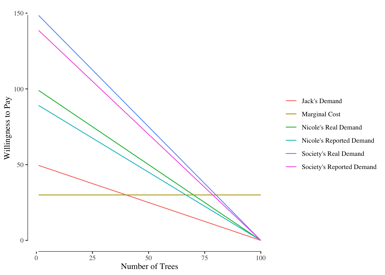
Based on the reported willingness to pay, it appears that the societal preferred quantity of shade trees would be 78 trees. At 78 trees, Jack’s demand is $11 while Nicole’s reported demand is $19.80. With the new marginal willingness to pay, Nicole saves $55.60 (80 trees at $20 versus 78 trees at $19.80) lowering her total cost by 3.5% while only reducing the number of trees planted by 2.5%. By under reporting her willingness to pay, Nicole lowers her total cost, shifting more cost onto Jack, at a rate faster than the reduction in the overall level of the public good provided. In large groups, any individual has an incentive to understate their preference for a public good because the quantity reduction will be more than offset by the price reduction.
Second, even when people are telling the truth, there are often problems for people placing a value on public goods. Abstract or large scale public goods, like national defense or fire prevention, are difficult for a person to value. Even goods that are less abstract but that we do not generally “buy” may be hard to value. I have no idea what the value I place on a single shade tree on my block is because I’ve never bought one.
Third, even when people are telling the truth and know the value of the public good, we might have a hard time figuring out the value that people assign to different levels. In our example, we just have Jack and Nicole, but in the United States, we have 320 million people. The government has no practical way of knowing the demand curves for each of the 320 million people and, therefore, has no hope of using Lindahl pricing to determine the correct levels of a public good.
These limitations mean that Lindahl pricing is rarely used in actual governance. The barriers to measuring peoples preferences over a range of prices and different goods make it a useful model but an impractical guide.
Instead, governments tend to use one of two major approaches to determining the socially desired level of public goods and policy approaches: direct democracy and representative democracy.
10.2 Preference Aggregation Systems
The Lindahl pricing model assumes that everyone agrees with the outcome and everyone is fine paying the taxes proposed by the government. In general, this does not happen unanimously but instead some people are displeased with the outcome. We instead need to find some other mechanism for aggregating preferences and turning the population’s preferences into policy choices.
In the aggregation mechanism, we want to consistently aggregate the voters’ preferences into a policy outcome. In order for that to happen, our mechanism must have three traits:
Dominance: if all voters prefer one of the policy options, it must return that policy option as the one selected by voters.
Transitivity: suppose we have three policy options: A, B, and C. If \(A \succ B\) and \(B \succ C\), then \(A \succ C\).
Independence of irrelevant alternatives: suppose the A, B, and C options are ideas for new bus routes and we have the ordering \(A \succ B \succ C\). If I include another item on the ballot, say a proposal to build a small park, it should not cause that ordering to change as it is unrelated to the question addressed by the policies A, B, and C.
Generally, voting schemes such as direct democracy (everyone votes on all issues) and representative democracy (everyone votes for representatives who vote on the issues) meet these requirements.
10.3 Direct Democracy
In a direct democracy, every policy choice receives a vote by the public and the majority vote rules. While the United States and many other countries do not make extensive use of direct democracy in favor of representative democracy, direct democracy is a facet of many state and local elections. Several states, most notably California, Colorado, and Oregon, allow for direct voting on policy proposals and make provision for the general public to act as a law making body. Local issues, such as local option sales taxes, property taxes, and bonds are often put to a popular vote referendum. While this approach seems like a good system for aggregating preferences, it is not without limitations and assumptions.
10.3.1 When Majority Voting Works
Suppose the City of Iowa City is considering implementing a local option sales tax (LOST) to fund expanding the bus system. The LOST is a sales tax paid to the city (typically, sales taxes are collected by the state and the county, not the city) on all sales within city limits. In Iowa, some large cities have LOST of 1% to pay for various services or improvements. Let’s suppose Iowa City has three options:
- LOST of 0% (e.g., not implementing a LOST) and leaving the bus network as it is,
- LOST of 0.5% and running the buses more frequently (e.g., lines that run every hour now are every 30 minutes, lines that run every 30 minutes are now every 15),
- LOST of 1% and running the buses more frequently and running more bus routes reducing walking to/from bus plus running later into the night/weekends.
Suppose Iowa City voters break down as follows:
- 1/3 drive everywhere they go and will never take the bus
- 1/3 walk or bike everywhere they go but sometimes take the bus if the weather is bad
- 1/3 take the bus everywhere they go
The person who exclusively drives will prefer the LOST of 0%. They do not want to increase the amount of taxes they pay for a service they don’t use. If they cannot get 0%, they would prefer 0.5% because it is lower than 1%. A LOST of 1% would be their least preferred choice.
The person who walks or bikes but sometimes takes the bus would likely prefer the LOST of 0.5%. They occasionally use the bus and when they use it, they want it to be easy to use and not have to wait for a long time for the bus to arrive. Their second choice is probably 0%. Their bus use is too occasional for them to want to a 1% tax for a full upgrade and given the choice between making the buses much better at 1% taxes or keeping them the same at 0%, they’d likely prefer 0%.
Finally, the person who exclusively uses the bus would prefer the 1% tax and the most improved service. If that isn’t an option, they’ll prefer the 0.5% tax and the 0% option the least.
We can put this in a table to summarize the three groups and their choices:
| Drivers | Walkers | Bus Riders | |
|---|---|---|---|
| First Choice | 0% | 0.5% | 1% |
| Second Choice | 0.5% | 0% | 0.5% |
| Third Choice | 1% | 1% | 0% |
We hold an election and the first question asks voters to select between a tax of 1% and a tax of 0%. We see that drivers and walkers prefer a tax of 0% to a tax of 1% and bus riders prefer a tax of 1% to 0%. A 0% option gets 67% of the vote and 1% gets 33%. We conclude \(0\% \succ 1\%\).
In the second question we compare the tax of 1% versus the tax of 0.5%. We see that drivers and walkers prefer 0.5% to 1% while bus riders prefer 1%. We have results where 67% of the voters select 0.5% while 33% select 1%. We conclude \(0.5\% \succ 1\%\).
In the third match-up, we compare 0.5% to 0%. We see that walkers and bus riders both prefer 0.5% to 0% while drivers prefer 0% to 0.5%. The results of the election are 67% selecting 0.5% and 33% selecting 0%. We conclude that \(0.5\% \succ 0\%\).
We can put these together to get an ordering of all three options. The first selection tells us that more people prefer 0% than 1%. The second election told us that more prefer 0.5% than 1%. We have two possible orderings of preferences based on those results, either \(0.5\% \succ 0\% \succ 1\%\) or \(0\% \succ 0.5\% \succ 1\%\). The last election tells us that \(0.5\% \succ 0\%\) and so we are left with \(0.5\% \succ 0\% \succ 1\%\) as the only possible ordering. This ordering also is transitive - no matter the order of the pairwise voting, we will always be left with this ordering. The city will always find the most support for a 0.5% LOST over all other options.
10.3.2 When Majority Voting Fails
Let’s revisit our example of residents voting on the LOST to expand the bus routes but add some complexity to our voters. Let’s suppose that drivers on the bus routes might change their choice to drive or take the bus depending on the level of service.
The drivers still prefer to drive and so their first choice is going to be a LOST of 0%. However, if they cannot get a LOST of 0%, they want a LOST of 1% and a full expansion of the bus route. They reason that if they have to pay the LOST to fund expansion of the bus route, they will drive less and use the bus instead to save money. Therefore, they want the bus possible system. Paying the middling tax of 0.5% for a middling improvement is a worst-of-both-worlds situation: they are paying more in taxes but the buses aren’t as nice as they could be. This changes the voting behavior of the drivers.
The walkers and the bus riders stay with their initial ordering of preferences for the different policy options. The new choice orders are summarized below:
| Drivers | Walkers | Bus Riders | |
|---|---|---|---|
| First Choice | 0% | 0.5% | 1% |
| Second Choice | 1% | 0% | 0.5% |
| Third Choice | 0.5% | 1% | 0% |
So what happens when we hold our elections?
We first ask about the 1% option versus the 0% option. We see that drivers and walkers prefer 0% to 1% while bus riders prefer 1% to 0%. The 0% option wins.
We then ask about the 1% option versus the 0.5% option. We see both drivers and bus riders prefer 1% to 0.5% and so 1% wins.
We hold our third pairwise matching of 0.5% versus 0%. We see that drivers prefer 0% while walkers and bus riders prefer 0.5% and 0.5% wins.
Putting this together, we see that \(0\% \succ 1\%\) and \(1\% \succ 0.5\%\). So far, so good. However, the third election tells us that \(0.5\% \succ 0\%\). This is a problem because the first election tells us that 0% was better than 0.5% and the second election told us that 1% is better than 0.5%. Those elections mean that 0.5% must be worse than 0% but the third election tells us otherwise. No matter what we do, a majority voting system will not arrive at a consistent result.
10.3.3 Arrow’s Impossibility Theorem
The problem described above is not with the voting system - majority voting certainly can work - but rather with the voter’s preferences. Indeed, other voting schemes like ranked choice voting (list the options from best to worse) will still yield inconsistent results.
The problem we face is one described by Arrow’s impossibility theorem. Kenneth Arrow first articulated this idea in his doctoral thesis and 1951 book Social Choice and Individual Values. Fundamentally, it says no voting system can meet the requirements we described earlier of dominance and transitivity unless
- We put restrictions on the allowed preferences or
- We have a dictator.
If we have a dictator, we only have one voter and therefore whatever the dictator wants is also the result of the “election.” Most of the time, however, we have many voters and the first element of the theorem is more important.
Specifically, our elections will fail to produce consistent outcomes when preferences are not “single-peaked.” Single-peaked preferences mean that not only do people have a first choice on the policy but their utility moves down as we move further away from their policy preference in either direction and never increases. Our groups in the first example have single peaked preferences, see Figure 10.1.
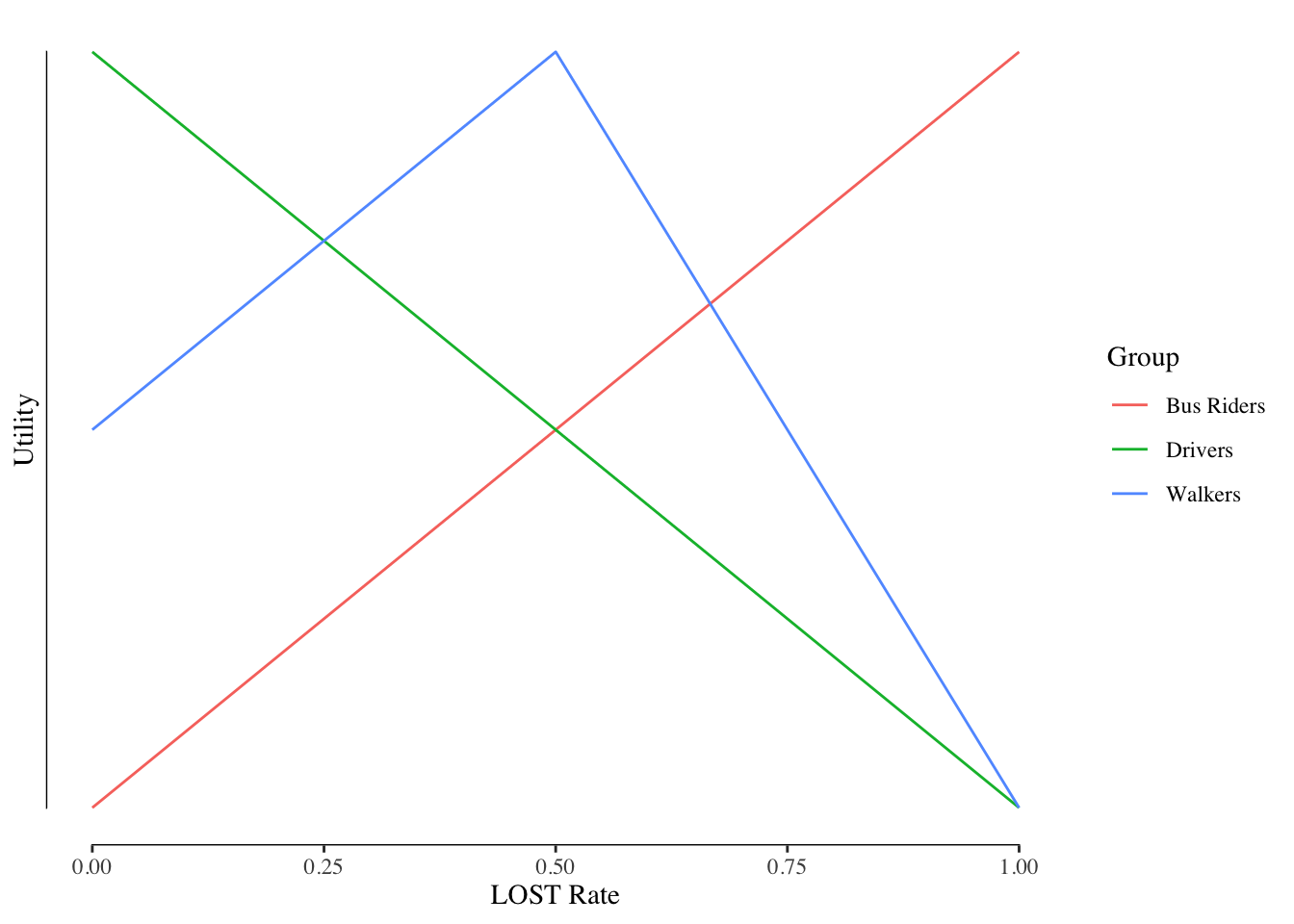
Figure 10.1: Example of Single Peaked Preferences
You’ll notice that for the bus riders all LOST rates that move towards zero have lower total utility. Likewise, all LOST rates that move away from zero have lower total utility for drivers. For walkers, there is one peak at 0.5% and it diminishes as we move either towards or away from 0.5%.
Our second example, however, has double peaked preferences for the drivers, Figure 10.2. Here, the preference curve for the drivers group is “V” shaped and increases as we either decrease the LOST from 0.5% or as we increase the LOST from 0.5%. The fact that it has more than one peak means that our population will never reach a consistent outcome through voting.
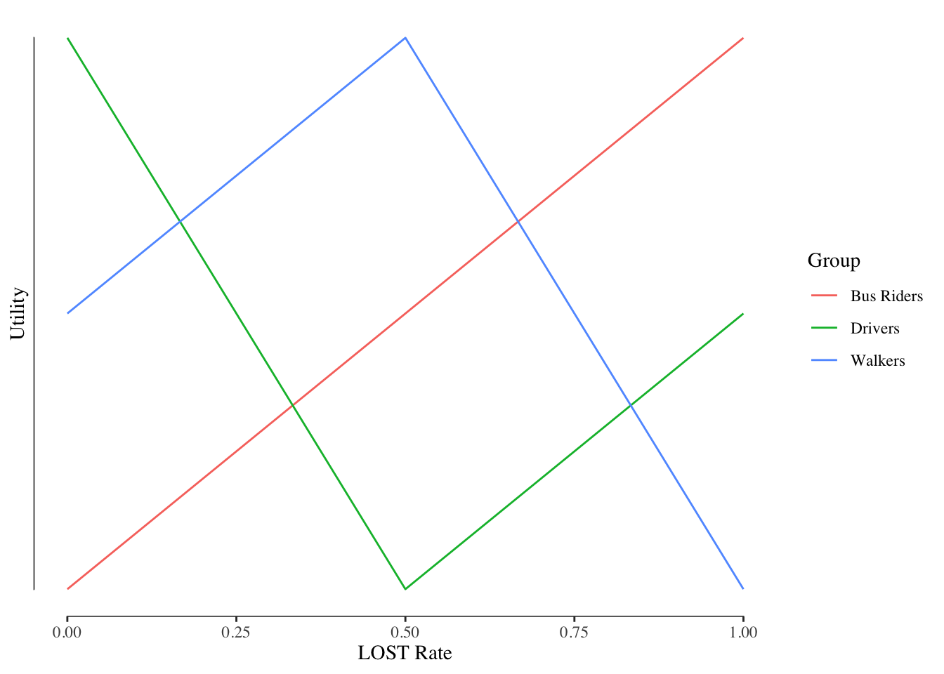
Figure 10.2: Example of Double Peaked Preferences
Multi-peaked preferences can happen. Our example here of the bus routes is a plausible case where it could be seen: the drivers don’t want the buses but if they have to have the buses, they want to the best. Parents of children attending private schools may feel the same about property taxes (that fund local public schools). They don’t get any value from the public schools when their children attend the private school and so prefer very low property taxes. However, if you increase the property taxes they would want the school to be very good so they can stop sending their child to the private school. However, in most cases, it is reasonable to assume that preferences will be single peaked unless we have reason to expect otherwise.
10.3.4 Median Voter Theorem
The median voter theorem says that, under direct democracy, the preferences by the median voter will determine the outcome. This makes sense: suppose we have 9 voters, 3 of whom are drivers who want 0% LOST, 3 are bus riders who want 0.5% LOST, and 3 are walkers who want 0.5% LOST. The first vote for 0% LOST cancels out the first vote for 1% LOST. The second vote for 0% cancels the second vote for 1% LOST, and the third votes also cancel. We now have three votes left for 0.5%. Two of those votes “cancel” and the middle vote, the median voter, determines the outcome.
There is one major limitation to the median voter theorem in that it lacks any accounting for strength of preferences. Let’s suppose instead of a LOST, Iowa City was considering a flat tax levy of $50 per person to pay for expanded bus service. We have a population of 1001 people who are voting on the outcome. Of the 1001 people, 500 would value the expanded bus service at $125 while the other 501 would value it at $10. The median voter, the voter where 500 people want more spending and 500 people want less spending, would value the expansion at $10 and therefore would vote “no” on the $50 tax.
However, the 500 people who valued it at $125 would have got \(501 * 125 = 62,600\) dollars in value from the expansion and the 501 voters who valued it at 10 dollars would have gotten \(501 * 25 = 5,025\) dollars in value. The total benefit of the buses would have been \(62,600 + 5,025 = 67,625\) dollars at a cost of \(50 * 1001 = 50,050\). This reflects a net benefit of $17,575. Society should want to expand the buses as the benefits of the public good are less than the cost; however, since the median voter was unwilling to pay $50, the system is left as is.
10.4 Representative Democracy
Most governments do not engage in direct democracy. It is relatively inefficient for everyone to vote on every issue and logistically challenging. It is often easier to have a representative democracy. In an representative democracy, the public elects officials to serve in a government and represent their particular interests.
There are two major forms of selecting representatives in a representative democracy. They are either “winner-takes-all districts” or proportional representation.
10.4.1 Winner-Take-All
Winner-take-all districts are the norm in most English speaking locations. Countries or regions are divided into small districts that each then select a representative of that district. The candidate that holds the most votes in that district after an election will represent that district. There are potential issues with such a system - we will discuss the most famous issue of gerrymandering later - but the biggest issue is that minority parties in a winner-take-all system do not get any representation. There are two major concerns with this.
First, it tends to lead to two major parties and no viable third parties. Suppose a district is voting and has three possible political parties that can represent the district and the voting in the first election has the following results:
| Color | Percent of the Votes |
|---|---|
| Red | 24 |
| Orange | 15 |
| Purple | 20 |
| Yellow | 15 |
| Blue | 26 |
The parties are listed in order of similarity (e.g., Orange is more like Red than Blue). We see that Blue wins the election with 26% of the vote. Most voters did not want Blue with 24% wanting Red and 50% wanting something in the middle.
As we head into the next election, Orange voters remember the results from before and their preference for Red over Blue and most vote for Red in the new election.
| Color | Percent of the Votes |
|---|---|
| Red | 34 |
| Orange | 3 |
| Purple | 22 |
| Yellow | 15 |
| Blue | 26 |
Red wins decisively after the Orange voters split. The Orange party, barely getting any votes, drops out before the next election.
Now the pattern repeats. Yellow voters prefer Blue to Red and so split, shifting most of their votes to Blue. The third election results are:
| Color | Percent of the Votes |
|---|---|
| Red | 35 |
| Orange | 0 |
| Purple | 27 |
| Yellow | 2 |
| Blue | 36 |
Blue wins this election. Some Purple voters realize that their views are more aligned with Red than Blue and shift their votes going into the fourth election. The Yellow party also folds after their terrible results. The fourth election results are:
| Color | Percent of the Votes |
|---|---|
| Red | 47 |
| Orange | 0 |
| Purple | 16 |
| Yellow | 0 |
| Blue | 37 |
Red wins by a significant margin. Purple voters closer to blue realize that their failure to support Blue over the non-viable Purple party defect to Blue for the fifth election.
| Color | Percent of the Votes |
|---|---|
| Red | 47 |
| Orange | 0 |
| Purple | 4 |
| Yellow | 0 |
| Blue | 49 |
Blue wins narrowly. As a result of the low vote share in the last election, Purple will fold and their voters will shift towards the party that is closest to their views.
As a result, third parties are forced out of the elections because their voters engage in strategic voting for the party nearest their preferences. Third parties also cannot enter the elections because votes for the third party candidate tend to harm the “mainstream” candidate more near those voters’ preferences.
Second, voters of the minority party do not get any representation. In Iowa, in 2018, there were 664,676 votes for Democratic candidates for the US House and 612,338 votes for Republican candidates for the US House. The Democratic party holds three of Iowa’s four seats despite winning only 50.52% of the vote in 2018. It is not clear that this is a “fair” outcome, it certainly does not represent the vote share of the two parties in Iowa. In other states, such as Wisconsin, this imbalance is even more stark. In 2018, Democratic candidates won 53.18% of the votes in Wisconsin but only controlled 3 of the 8 (37.5%) of the seats.35 Some level of imbalance is expected because only one person can represent a district at a time; however, winner-take-all systems can exaggerate the imbalance.
10.4.2 Proportional Repersentation
A common voting common in non-English speaking countries is proportional representation. Unlike a winner-takes-all system with one member per district and relatively small districts, proportional representation has larger districts with a greater number of representatives per district. The most common form of proportional representation is “party list proportional representation.” Under a party list proportional representation scheme, voters either select candidates off a list or vote for their preferred political party and the political party then decides who fills the seats they win.
Proportional representation can improve on winner-takes-all system in two important ways.
First, the composition of the representative body more closely resembles the voters’ preferences. Using Iowa’s 2018 House election as an example, there were 4 seats being challenged and Democratic candidates won 50.25% of the vote and 75% (3) of the seats. This an “unfair” result in that barely half of Iowans voted for Democratic candidates and the 75% of the seats won does not reflect that. Under a proportional representation scheme, Iowa might pool the votes across the state and award the four seats according to the results. In that case, in 2018, Iowa would have likely awarded two seats to both parties reflecting the nearly equal vote share. As a result, the percent of votes won by a party and the seats held are generally very similar.
Second, this creates room for minor parties. A risk voters take in winner-take-all system is that any vote not for one of the major two parties is likely to be “wasted” as the candidate has no chance of winning. Any votes for candidates with near-zero chance of winning are wasted in the sense that the vote does not influence who wins the district. Under a proportional representation system, that vote would count towards the parties support. In relatively large districts, this allows minor parties a foothold in the representative body. This ensures that smaller or less-mainstream voices are heard in the political process.
There are some drawbacks to a proportional representation voting scheme. Often, the largest party in a proportional representation voting scheme will not gain a majority of the seats and, therefore, typically cannot be the majority party in the government. In situations where this happens, the small parties can be asked to join in “coalition” with the larger party to set the size of the coalition over 50% of the seats. The smaller parties ask for concessions from the larger party in exchange for joining the governing coalition. This can create a government that may give the smaller groups greater influence than their vote share would warrant or increase government instability.
This is doubling a concern as the small parties may reflect extreme political positions not supported by the mainstream voters. For instance, Israel is often plagued with issues building a governing coalition as voters and the larger parties reject more extreme positions but too few people vote for the major parties to let them create a government without a coalition. More geographically isolated and nationally-fringe groups, like Bloc Québécois, the Scottish National Party, or the UK Independence Party may not reflect national interests but may be required to form the governing coalition. Some systems, notably the German Bundestag, have a threshold number of votes a party receive before it is giving a seat. This increases stability and reduces the number of extreme parties, but comes at the cost of the system more closely representing the problems of winner-takes-all.
10.4.4 Assumptions of the Median Voter Theorem
The median voter theorem is an abstraction and a model of a complex system. It provides powerful insights into why government choices are the choices that they are and how electoral systems influence outcomes. However, as an abstraction, we necessarily have to make a number of limiting assumptions in order for the model to make sense. Some of these assumptions are generally met while others are honored in the breach.
We chiefly focus on six major assumptions: voters are single-dimensional, there are only two candidates, there is no ideology, everyone votes, elections are costless, and there is full information.
10.4.4.1 Voters as Single-Dimensional
We assume that voters are making their decision on only one issue and not a combination of issues. If there are several issues then a vote maximizing politician might select a location that is vote maximizing but not always the median voter’s preference on that issue. See a plausible example with voters over two dimensions in Figure 10.3.
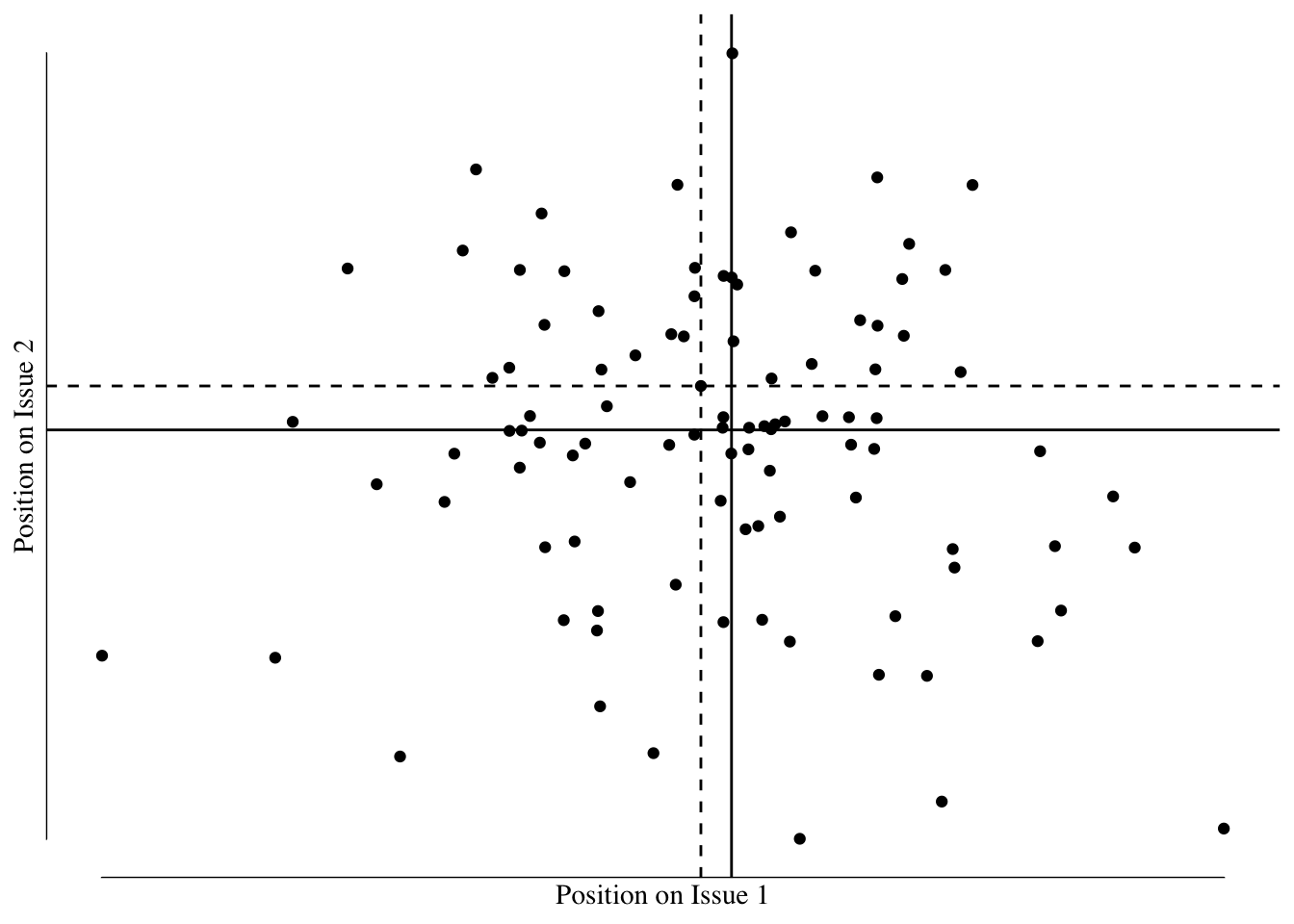
Figure 10.3: Example of difference between the single dimensional median voter positions (black solid lines) and the median voter over two issues (dashed lines).
Because the voters are voting on several issues, the median voter on the bundle of issues might hold a different position than the median voter on any single issue. As a result, a vote maximizing politician might select a position that does not reflect the median voter on any given issue.
Rarely do we as voters ever have the option of voting for a politician based exclusively on a single issue. As a result, it might seem like this assumption is violated in nearly every election. However, in practice, it tends to be pretty reasonable. Politics in the United States and elsewhere has become increasingly polarized and our political views increasingly tied together as a bundle of positions. We’ll talk more about polarization in a following section but the primary result of polarization is an alignment of our personal views with that of the party with which we identify the strongest. This results in our voting options becoming increasingly single-dimensional.
10.4.4.2 Only Two Candidates
The median voter theorem only provides a solution where there are exactly two candidates in the race. If there are three or more, there is no stable position that maximizes vote share for the candidates. To see why this is the case, imagine we have three candidates that all support a 0.5% LOST. Each of those candidates would get a third of the vote. However, if one of the candidates shifted her position to be in favor of a 0.51% LOST, she would capture ALL of the voters who support a 0.51% or higher LOST while losing only the voters who preferred a LOST of 0.50% or less. Before shifting, she captured a third of the vote but by moving she captures just under half (1/3 of the voters between 0.50% and 0.51% and all the voters from 0.51% to 1%). It is always better for a candidate to take a position just below or just above the other candidates if there are three or more candidates for the office.
On the other hand, if there are exactly two candidates, shifting their position to just above or just below the other candidates position will decrease the total votes gained. As a result, politicians stay on the median position where there are exactly two candidates.
In the United States, practically speaking, there are two political parties: the Republicans and the Democrats. While there are other parties (major third parties like the Libertarian and Green parties and more minor third parties like the American Solidarity Party), these third parties are rarely, if ever, viable candidates for election. As a result, the majority of the voters and the politicians making positions ignore these voters. The assumption of two parties or two candidates is generally a reasonable one in the United States.
10.4.4.3 No Ideology
In the median voter theorem, we assume that candidates for office review the preferences of the voters in their district and then select a position that roughly reflects the median voter, whatever that position is. For instance, if the median voter prefers a 0.5% LOST rate, both the Democratic and Republican candidates should argue for a 0.5% LOST to maximize their vote share.
However, generally, the two candidates balance what the median voter wants with their party ideology. As a general rule, Republicans want lower and fewer taxes while Democrats want higher and more taxes. As a result, the Republican candidate might take a position below 0.5% LOST rate reflecting the party ideology that higher tax rates are bad. The Democrat might take a position at or above 0.5% reflecting the party ideology that the services provided by the tax returns justify increasing the tax. In both of these cases, the party ideology pulls the candidates away from the location of the median voter.
10.4.4.4 Everyone Votes
The figure below shows the percentage of Americans asked by Gallup whether they preferred that immigration rates be increased, remain the same, or be decreased.36.
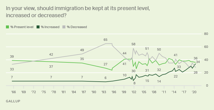
img
In 2016, roughly 21% of voters thought it should be increased, while 38% would prefer no change and 38% wanted a decrease. The majority (59%) wanted the rates of immigration to either increase or stay the same. The median voter would have preferred immigration rates stay the same.
The numbers supporting expanded immigration increased by 2020 with 34% supporting expanded immigration, 36% keeping the numbers about the same, and 28% wanting a decrease. The majority (70%) wanted numbers to either remain unchanged or be increased and the median voter again preferred rates stay constant.
In both the 2016 and 2020 election cycles, however, the Republican candidate, Donald Trump, ran on a strongly anti-immigration stance. During his first term between 2017 and 2021, barriers to legal immigration increased. Given that this position does not reflect the median voter’s preferences, why did Trump run on this stance and how did he get elected?
Increasingly, who wins elections is not about taking the position that maximizes the number of people who vote for you but rather taking the position that maximizes the number of your supporters who show up to vote. Trump’s position created a high level of energy among the roughly 1/3 of the population who opposed even existing levels of immigration and brought them out to the polls. While this position only reflected the preferences of a third of the population, by bringing them out to the polls in high numbers it was a better approach than trying to win by maximizing the total vote share.
The median voter theorem avoids this problem by requiring that all eligible voters vote. When all voters vote, the median voter is the vote that determines the outcome. However, if only a selection of voters vote, the outcome will not reflect the median voter’s preferences. This assumption is almost always violated. In the United States during presidential election years (midterm elections generally have even lower turnout) turnout rates are around 50% to 60% of registered voters. Voters who turn out tend to be older, more highly educated, and with greater incomes than voters who do not vote. As a result, the outcome of the election reflects the median voter of this selected cohort, not of the total population.
Low turnout is sometimes used by politicians to increase their advantage or help determine results. We’ll discuss the effects of turnout in a upcoming section.
10.4.4.5 Running for Office is Free
The median voter theorem assumes that candidates for office take positions that reflect the median views of the voters in order to maximize the probability of winning an election. However, running for and winning office is generally an extremely expensive proposition. The cost of winning a seat in the US House of Representatives is over 1.5 million dollars and the cost for a Senate seat is nearly 10 times greater. Therefore, candidates must expend a significant amount of time and energy fundraising for their campaign. Candidates must consider the preferences of donors to the campaigns and take positions that might not be vote maximizing but are needed to ensure that the candidate will be able to raise enough money. The median voter theorem assumes that running for office is free and therefore candidates do not need to consider the position of donors or other non-voters in their position. This is likely not a realistic situation in American politics.
10.4.4.6 Full Information
The last assumption we’ll consider is probably the most egregiously violated. We assume that candidates for elected office have full information about voter preferences, that is they know exactly what voters want, as well as having a full understanding of the issues they are voting on. We also assume that voters have a full understanding of the issues and the politicians’ positions on the issues. Given the complexity of the laws as well as the future regulations written to define the rules, no one has a full understanding of the issues.37
https://www.theatlantic.com/international/archive/2015/09/welfare-reform-direct-cash-poor/407236/↩︎
https://www.brookings.edu/testimonies/pros-and-cons-of-restricting-snap-purchases/↩︎
https://www.ncsl.org/research/human-services/drug-testing-and-public-assistance.aspx↩︎
https://www.theatlantic.com/international/archive/2015/09/welfare-reform-direct-cash-poor/407236 and https://www.brookings.edu/testimonies/pros-and-cons-of-restricting-snap-purchases/↩︎
https://www.clasp.org/publications/fact-sheet/drug-testing-and-public-assistance↩︎
Wisconsin is somewhat infamous for the imbalance and in 2018 was the only state where this was true. Wisconsin maps feature relatively high levels of gerrymandering and voter concentration, resulting in this imbalance. In Iowa, our district maps are drawn by a bipartisan panel and are explicitly not supposed to be the subject of gerrymandering. The maps in Wisconsin are drawn by the state legislature and explicitly feature gerrymandering. The boundaries are drawn every 10 years and Republicans had taken control of Wisconsin’s state house in 2010. Democratic senators from the state “hid” in Illinois to prevent the Republicans from having the votes to pass the new maps for a period of time. Ultimately, the maps were passed. Legal challenges to the maps have gone up to the United States Supreme Court; however, thus far there has been no favorable ruling to people seeking to reduce the impact of gerrymandering on election results.↩︎
Source: https://news.gallup.com/poll/1660/immigration.aspx↩︎
Laws that are passed by Congress are generally codified into regulations by the executive branch. The number, and relevance, of these rules and potential crimes that you could be committing is outstanding. The Twitter account
CrimeADayhighlights one humorous potential crime each day from the US Code. The crime for today, as I write this, is “a federal crime for a department of agriculture employee to reveal how a watermelon handler voted in a watermelon referendum.”↩︎