Chapter 6 Solutions to Externalities

The root cause of externalities is the divergence between the societal and private costs or benefit functions. If \(\text{SMC} = \text{PMC}\) and \(\text{SMB} = \text{PMB}\), there is no problem with the free market solution. This suggests if the cost (or benefit) of the transaction can be “internalized” to the firm or consumer making the decision, then the externality would be addressed and the free market competitive equilibrium and the socially optimal equilibrium will converge. We have two major options for reaching this goal: private market solutions or governmental action.

6.1 Private Market Solutions

In standard economic theory, the market is considered to be efficient and effective at reaching the best outcomes. Indeed, unless we have evidence to the contrary, we assume that markets reach the best and most efficient outcomes. Therefore, it is reasonable to assume that there is some private market solution to externalities.

Robert Coase, an economist and lawyer at the University of Chicago, attempted to provide a framework for these solutions and his answer is formalized as the Coase theorem. The Coase theorem has two parts and basically says clear assignment of property rights to either party provides an opportunity for a market-based solution to the externality.

Consider the example of the Des Moines Water Works (DMWW) dealing with high nitrate levels in the water due to agriculture runoff in the watershed of the Raccoon River. Let’s suppose each additional 100 acres that are farmed result in the DMWW needing to spend an extra $5 on water treatment. We would then have \(\text{SMC} = \text{PMC} + 5\) per 100 additional acres being farmed.

6.1.1 Coase Theorem Part I

What happens if the DMWW owned the river?

The answer is simply - they could demand that the farmers in the Raccoon River watershed change their practices to avoid excess levels of nitrogen ending up in the river. If the farmers failed to alter their practices, the DMWW could sue the farmers, as the DMWW owns the rights to the river, and force them to either pay for the damages they do or change their practices.

Let’s suppose DMWW is equally happy to be paid to remove the nitrates or to not have to remove them in the first place. In other words, the DMWW would be equally happy to spend $5 treating water or by having 100 fewer acres being farmed and saving them $5 on water treatment. Either way their position is unchanged.

How would imposing this cost on the farmers change their marginal cost? Now, each additional acres they farm would come with an additional $5 cost paid to the DMWW. Because of this change to their PMC function associated with internalizing the cost of the harm to the producers, the firm’s cost function is now the same as the SMC. As a result, the competitive market would now clear at the socially optimal location.

This leads to the first element of the Coase theorem: when property rights are clearly defined and there is costless bargaining, negotiations and transfers between the party creating the externality and the party experiencing the externality will shift the market to the socially optimal quantity and price. This is easiest to think about with pollution or related externalities. If one of the two parties owns the right to the air, water, or ground, they can use that property right to demand a solution to the externality. By having clearly defined and established property rights, the party that was “external” to the initial trade now has the ability to influence the trade through those rights.

6.1.2 Coase Theorem Part II

Where the Coase theorem gets interesting is the realization that who owns the property rights does not matter. Above, I assumed the DMWW owned the rights to the river and therefore could demand that the farmers stop polluting. However, what would happen if the farmers owned the river?

The farmers are equally happy farming an extra 100 acres or being paid not to farm that land so long as the net impact on their income is zero. The DMWW is equally happy paying the farmers to reduce their pollution as they are to remove the nitrates from the water.

Suppose that the DMWW was willing to pay the farmers $5 per every 100 acres they did not farm (e.g., the marginal damage from farming that 100 acres). This would introduce a new input into the cost function for the farmers. Previously, the marginal cost function for the factory was just the increase amount of labor required to farm the extra 100 acres. This is the value of the PMC curve. However, when the DMWW offers $5 per 100 acres not farmed, the PMC curve is increased by $5 - each time the farmer farms an extra 100 acres, they have to give up $5 in payments. Since they are forgoing that income, it is coded as a cost to the farmers.

This results in the cost of the externality being internalized to the farmers. The SMC and PMC curves are now the same resulting in the market moving to the socially optimal location. This is the second part of the Coase theorem: the assignment of the property rights can be to either party.

6.1.3 Limitations of the Coase Theorem

While the Coase theorem does provide an elegant market-based solution to the problems of externalities, it has several limitations. The four biggest issues are problems of assignment, hold outs, free riding, and transaction costs.

6.1.3.1 Assignment

Suppose you are in your apartment, being a good student, on a Wednesday night and the people across the hall are having a very loud and large social gathering. This is a negative consumption externality - the loud music of their gathering is negatively affecting your studying. It is pretty clear who the party responsible for the externality is (the person playing the music and hosting the party), who are the parties that are adversely affected (those living near the apartment), and the extent of the damage (however much the music interferes with their ability to study).

But most real world problems aren’t so easy. Consider the case of the DMWW and the farm runoff. It is easy to identify who is harmed (DMWW) and how much (how much money is spent on the nitrate removal facility) but it is difficult to identify who is doing the harm. Many farmers are engaging in farming practices, so assigning harm to any particular farmer may be difficult. Different farmers use different amounts of nitrogen, tiling, or runoff control practices, so assigning the exact portion of blame to each farmer may be difficult.

The same is true when the person doing the harm is clearly identified but the number harmed is quite large. Legionnaires’ disease is a type of pneumonia caused by bacteria of the genus Legionella. In order to infect us, the bacteria must become suspended in the air in some water droplet. One common route is through shower heads splitting the water into a many streams and some of the droplets that come out are very small. However, these droplets are also frequently generated by large cooling towers used as part of the air conditioning system of large buildings - you can see one of these towers along the parking ramp on Newton Road. These towers can create small droplets that easily can travel several miles on the wind. While the source of many droplets can easily be identified, it might not be possible to identify those harmed. Even among people with Legionnaires’ disease, it may be that they were infected while taking a shower or swimming and not from the cooling tower.

The difficulties in assigning “blame” or “harm” to specific actors and measuring the level of harm result in difficulties in resolving the externality through the Coase theorem.

6.1.3.2 Free Riding

Imagine we have a circumstance where a factory is dumping waste water into a river and that is harming the community downstream, in particular the farmers and ranchers. The farmers agree to each pay $100 to the factory and the factory would reduce the waste output (remember the farmer paying $100 to the factory shifts the factory’s PMC curve by $100). The farmers arrived at this number because the emission from the factory was costing them each $100 in reduced yield.

Let’s suppose there are 100 farmers that are part of this pact. The first 99 farmers agree to pay, what does the last farmer do?

If the last farmer pays his $100, there is a 100 unit reduction in the pollution and he gets $100 increase in his yield. But, if the last farmers decides not to pay, he saves $100 and, since the other 99 farmers have paid, the factory reduces emission increasing his yield by $99. When the farmer pays, he gets $100 increase in yield at the cost of $100. If the farmer does not pay, he gets 99% of that increase in yield, or $99, at zero cost. The rational farmer would then decide to not pay - by not paying he earns $99 but if he does pay he has a marginal gain of $1 at the cost of $100.

The 99th fisherman will notice this and may elect to not pay - he also stands to gain by letting others pay and getting a somewhat smaller benefit for free. This process will repeat over and over again. This is called free riding and happens whenever the investment has a common benefit (extra yield to all the farmers) but comes with a personal cost (the payment made to the factory).

6.1.3.3 Hold Outs

Imagine instead the factory agreed to pay each farmer $100 to offset the reduced yield from the pollution and until each farmer agreed to accept the payment, the factory couldn’t release the waste water. The first fisherman takes the $100 and moves on. This process continues for the 2nd, 3rd, and so on farmer.

Now we get to the 100th farmer. The prior 99 farmers all agreed to accept the payment and all the waste to be emitted and the factory has obligated itself to pay $9,900 to those farmers. The final farmer needs to agree in order to allow the factory to release the waste. What does she do?

The farmer will likely realize that she has leverage over the factory - until she agrees, the factory cannot pollute and they’ve already spent nearly $10,000 on this agreement. She could demand a payment larger than the $100 of harm she suffers because the factory really wants her permission. She may hold out and demand a larger payment and the factory will almost certainly grant her the extra payment.

However, the 99th farmer sees this process and now refuses the offer in an attempt to be the last payoff. The earlier farmers also see this and attempt to be a later, if not the last, payoff in order to demand a higher payment from the factory. As a result, no deal can easily be made.

6.1.3.4 Transaction Costs

The first three problems are issues because the number of parties is large. It is unclear who is doing the harm, who is harmed, the extent of the harm, and, because of the large number of parties, there is incentives for free riding and hold out behavior. The final problem exists even when the number of parties is small. The Coase theorem assumes no transaction costs or negotiation problems - the “costless bargaining.” This is almost never true.

Consider the situation of the loud party - the idea is simply, you can to the party host and either offer them payment to stop the music or demand payment to allow the music depending on the property rights. But that is awkward. Even though the number of parties is small, the negotiation is not costless.

When the number of parties is large, like in the example with the farms and the DMWW, it might not be possible to effectively bargain with the parties. The DMWW would have to identify and engage directly with hundreds or thousands of land owners and farmers in that case. It simply isn’t practical.

The Coase theorem works best when the number of parties is small, the harm is clearly identified and measured, and the parties are of relatively equal status. When there is a different in status between the parties and one party can exploit that, the negotiations are unlikely to meet the requirements of the Coase theorem. When the number of parties is large, the costs associated with the bargaining are very high. If the harm is not clearly identified and measured, disputes over the extent and relative apportionment of the harm may derail negotiations.

Since most externalities of serious public health concern (e.g, pollution, climate change, infectious diseases, antibiotic resistance) tend to have very large numbers of potentially poorly identified parties, with significant risk of free riding or hold outs, the externalities may be best addressed through government action.

6.2 Public Sector Solutions

In the United States, the preferred solution to most large scale externalities has been government action instead of the more limited Coasian solutions. There are three major approaches the government can use to resolve externalities:

1. They can apply a tax on the production or consumption of the good to offset different because the private curves and the societal curves;
2. They can provide subsidies to increase consumption of goods with positive externalities or discourage consumption of goods with negative externalities;
3. They can use explicit regulations - such as putting a limit on the amount of pollution allowed from a power plant.

Each of these three approaches can achieve the desired outcome, although all differ somewhat.

6.2.1 Taxation

Corrective taxation is very similar to the Coasian solutions that internalize externalities; however, instead of the affected parties negotiating payments, the government imposes a tax on the production or consumption of a good. This tax is designed to internalize the negative effects to the producer or consumer and bring the production/consumption levels to the socially desired point.

6.2.1.1 Addressing Negative Production Externalities

Suppose the government wants to address the extra costs and health risks to people in Des Moines created by the higher levels of nitrates in the Raccoon River. They could impose a tax on each unit of fertilizer or tiling sold with the tax being equal to the marginal harm from that unit of fertilizer or tiling. Previously, the farmer’s marginal cost was simply the extra labor and inputs required to farm another acre of land; however, with the tax this is increased by the amount of the tax. Recall that in the case of negative production externalities

\[ \text{SMC} = \text{PMC} + \text{Marginal Damage} \]

By incorporating the marginal damage into the farmer’s cost function, the market will use \(\text{SMC}\) as the supply curve and now produce the lower \(Q_\text{SMC}\) amount of corn and soybeans.

6.2.1.2 Addressing Negative Consumption Externalities

A big issue in large, dense cities is traffic congestion. It takes a long time for people to travel by car from one point to another - often slower than walking. This is the result of a negative consumption externality as driving on a roadway is generally free but each additional car slows down all the cars. The \(\text{SMB}\) and \(\text{PMB}\) then differ for a person deciding to drive or take mass transit/bike/walk. They realize their personal benefit (comfortable seats in their car with music) but do not realize the harm it imposes on others attempting to use the same streets.

European cities, such as London and Stockholm, have started using a congestion charge and such a charge has been planned to enter the island of Manhattan. Essentially, this is a charge or toll imposed on any car entering the core areas of these cities - functionally a fee for using the roadway. Typical fees vary from place to place, and even across the day with weekends and evenings being cheaper than weekday days, but typically run around $15. This fee discourages “optional” driving but people who still need to enter the city by car (e.g., delivery, construction workers, etc) are allowed to enter with the fee. This has the effect of reducing traffic congestion so those who must drive can travel faster and reducing the amount of pollution in the city center from car emissions.

This fee works by adding a cost to the \(\text{PMB}\) such that the demand curve they will utilize is the \(\text{SMB}\) instead. By internalizing the marginal damage to the drivers, the demand for road space is decreased and the congestion reduced.

6.2.2 Subsidies

Corrective taxes are suitable for addressing negative externalities but do not have much of a role in addressing positive externalities, such as tree planting, mask wearing, proper antibiotic use, or getting vaccinated. To increase the these activities, the government can use subsidies²³ to reduce the cost of the activity they want more of.

6.2.2.1 Positive Production Externalities

Consider the beekeeper example. The bees pollinate plants on nearby land, creating value for the land owners that is not realized by the beekeeper. As a result, there are too few beehives because the beekeeper uses her \(\text{PMC}\) function to determine her production. However,

\[ \text{SMC} = \text{PMC} - \text{MB} \]

and therefore society would prefer additional production of beehives.

One way they can do this is to provide a subsidy to the beekeeper equal to the \(\text{MB}\) of the beehive. This results in the beekeeper’s marginal cost function being decreased to the \(\text{SMC}\). As a result, she will increase her production of bees until we reach the socially optimal quantity.

6.2.2.2 Positive Consumption Externalities

Suppose the government wants to increase the uptake of vaccination, an action that has positive externalities through herd immunity. Without a subsidy, the consumer makes his decision based on \(\text{PMB}\) alone and ignores the marginal benefit to society from his actions. The government could issue a subsidy to the consumer to encourage this activity and, if the subsidy is equal to the marginal benefit to society, the consumer will use a demand curve equal to \(\text{SMB}\) instead of \(\text{PMB}\) when making decisions. This will increase the quantity consumed.

6.2.2.3 Can Subsidies Decrease Negative Externalities?

In the two examples, we discussed using subsidies to increase consumption or production of goods with positive externalities but can we use subsidies to decrease consumption of goods with negative externalities? For instance, gasoline powered cars contribute to climate change through their engine emissions and are a primary source of air pollution in cities. Can the government encourage the consumption of electric cars instead of using a tax on gasoline powered cars to fix the externality?

This makes sense - the government’s actions would create a cost on purchasing a gasoline car (requiring you to forgo the subsidy) and also creates an incentive to buy an electric car. This should increase demand for the electric cars and decrease demand for the gasoline powered cars. Indeed, federal and state tax codes often include incentives for purchasing electric cars over gasoline powered cars.

While this idea has appeal and may be politically easier than a tax on buying gasoline cars, it is typically less effective than just applying the tax directly to the thing we want to discourage for two reasons.

First, subsidies require the government to spend money (which it must raise through taxes or borrow as debt) while a tax will create revenue for the government. It is easier for the government to create revenue then to spend money in an effort to reach the same goal.

The second issue is the subsidization of alternatives is risk and the effect is uncertain. Consider the $7,500 tax credit for people who purchase electric cars.²⁴ This provides a tax credit, or a reduction of the federal income tax due, of $7,500 to people who buy an electric car regardless of the price of the car. If a person buys a $100,000 Tesla Model X, they a $7,500 reduction in their income tax bill. However, to what extent was the purchasing decision of someone buying a $100,000 car swayed by the $7,500 tax credit? It is likely that even without the tax credit, this person would still have bought the Model X.²⁵ The government would have spent $7,500 in this case and likely failed to achieve the intention of the program. It is much less risky and the effect more certain to simply tax the activity that we want to discourage.

6.2.3 Regulations

The above two methods are very similar to the Coase theorem approach but feature the government handling the negotiation and distributing/collecting the payments. However, a much more common approach has to be use regulation to ban or limit the production or consumption of goods that create externalities.

The chemical \(\text{SO}_2\) is by-product of combustion of fossil fuels. High levels can be toxic but even low-levels, with a long-term exposure, can harm human health. As a result, emissions of \(\text{SO}_2\) have been regulated in the United States through a scheme known as “cap and trade.” Under this program, firms are issued credits that can be exchanged for the right to emit \(\text{SO}_2\) or they can sell the credits they do not need to other firms that need more credits to cover their \(\text{SO}_2\) emissions.

Likewise, in response to a widening “hole” in the ozone layer around earth, largely caused by human emissions, especially of chemicals known as CFCs, most of the countries in the world banded together to strictly limit - in essence, ban - use of CFCs.

This approach has a certain appeal - we are simply restricting the amount of production/consumption so that the quantity produced is the socially optimal quantity. This is easier to define, easier to implement, and generally has been preferred by policy makers. However, economists argue strongly in favor or taxes or subsidies, so-called price approaches to addressing an externality instead of quantity approaches like caps.

6.3 Price and Quantity Based Approaches to Externalities

As mentioned above, there are two major approaches: regulating the quantity produced or regulating the price. Economists prefer price regulations, like taxes, over quantity regulations. To understand why, let’s focus on how each approach works.

6.3.1 A Market for Pollution Reduction

So far we’ve focused on the market that procedures the externality; however, there is a second market we can consider: the market for the reduction of that externality. Let’s take air pollution as our example externality. In your car, we can install a part called a catalytic converter that removed harmful \(\text{NO}_x\) gases from your exhaust and renders them into harmless compounds. We can increase the efficiency of the engine to require less fuel or we can make the car lighter to require less fuel per mile. We can convert a coal burning power plant to one that burns oil or natural gas, which, while still producing emissions, are significantly lower than when we burn coal. These changes can reduce air pollutants released without reducing output. We can imagine a market for these products.

The supply lines look like all of our prior graphs. The actual cost of installing a pollution reduction technology is the \(\text{PMC}\) and since the output is not reduced following this installation it is also the \(\text{SMC}\). This makes sense - the cost to Ford to install a catalytic converter on your car is the price of the catalytic converter and, since it doesn’t impair your use of the car at all, that is also the cost to society.

The demand side looks a little different. The marginal benefit to Ford for installing the catalytic converter is zero. Ford does not get paid more for installing this part and does not derive any particular benefits for doing so. As a result, the \(\text{PMB} = 0\) for all the values of \(Q\). However, society gets a benefit from Ford installing the catalytic converter through lower levels of air pollution. The extent of of the societal benefit is \(\text{SMB} = \text{PMB} + \text{MD}\), where \(\text{MD}\) is the marginal damage that is averted through reducing the pollution. Since \(\text{PMB} = 0\), the \(\text{SMB} = \text{MD}\).

An example of what this market would look like is shown in Figure 6.1. In this figure we assume that marginal damage of pollution is constant. Going from a particulate matter smaller than 2.5 microns concentration of 30 \(\frac{\mu\text{g}}{\text{m}^3}\) to 20 \(\frac{\mu\text{g}}{\text{m}^3}\) has the same benefit as going from 20 \(\frac{\mu\text{g}}{\text{m}^3}\) to 10 \(\frac{\mu\text{g}}{\text{m}^3}\). This isn’t likely to the case - most of the time human health decreases non-linearly with increased exposure levels. However, we’ll draw the line as if it where constant for ease and clarity.

However, the \(\text{SMC} = \text{PMC} = \text{supply}\) line is not flat but rather increases with increased reductions in the amount of emissions. This makes sense. In general, the first units of pollution reduction are cheap. Thinking about your car, you can easily improve the gas mileage by ensuring the tires are properly inflated, any excess weight is removed (e.g., taking out items instead of letting them ride in the trunk), spark plugs are new, and selecting more fuel-consumption optimal speeds. The improvement that comes from those steps is cheap and relatively easy. Bigger reductions could be made through swapping out metal parts with lighter metals (aluminum or carbon fiber versus steel) to reduce weight, redesigning the engine to increase efficiency, and making the car more aerodynamic. These changes would result in improvements but would be much more costly. Hence the supply curve in Figure 6.1 slopes upwards.

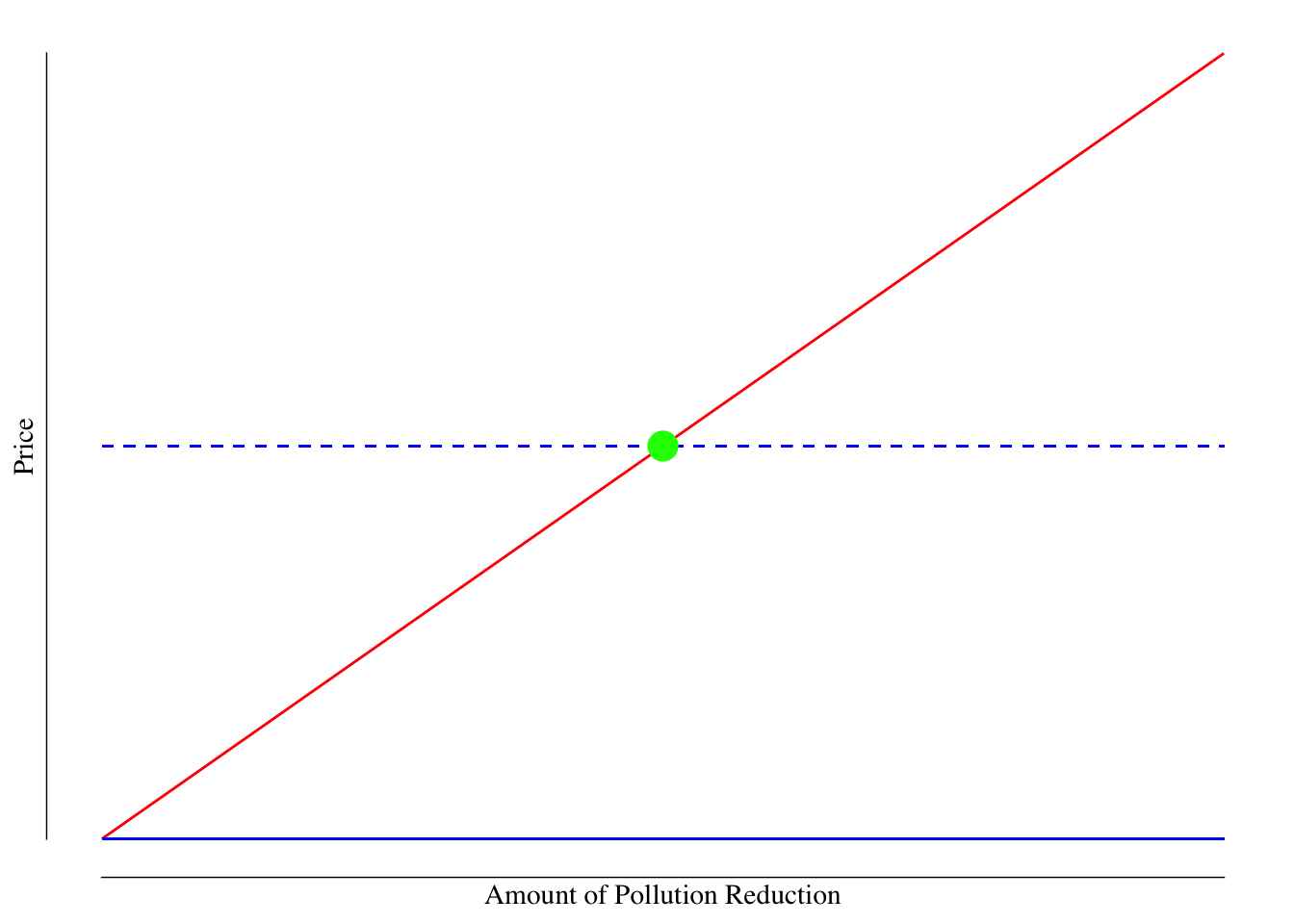
Figure 6.1: Market for Pollutation Reduction. The red line is the supply line ($ ext{SMC} = ext{PMC}$ while the blue lines are the $ ext{PMB}$ (solid) and $ ext{SMB}$ (dashed). The societial optimal point is shown as the green dot - this is the point where the cost of reducing pollution is equal to the harm averted by that reduction. Any additional reduction in pollution would cost more than the benefit to society while any less reduction would harm society more than it would cost to avert. The $ ext{MD$ here is assumed to be constant for simplicity; however, it could be curved reflecting non-linear harms of pollution.

Society would demand a reduction in emissions to to the point shown in green in Figure @(fig:market-for-reduction) at the intersection of the \(\text{SMB}\) and supply lines. This is the point at which any further reduction in pollution would not offset enough harm to society to be worth doing while any less reduction would harm society more than the cost to reduce the emission.

Suppose each ton of \(\text{CO}_2\) causes $40 worth of harm through climate change. The \(\text{MD}\) would then be $40. If it cost less than $40 to reduce \(\text{CO}_2\) emissions by one ton, we would reduce the \(\text{CO}_2\) emissions as we get $40 in benefit at less than $40 in cost. If it costs more than $40 to reduce \(\text{CO}_2\) by one ton, we would not make that reduction as the cost is greater than our $40 benefit. The point at which the cost of reduction is $40 and the benefit of reduction is $40 is optimal and is the intersection of our supply and \(\text{SMB}\) lines.

6.3.2 Market Response to Corrective Taxes

How would this market for pollution reduction respond to a corrective tax? Suppose the government was interested in creating a tax on carbon emissions equal to $40 per ton of \(\text{CO}_2\) (their best estimate of the harm per ton of \(\text{CO}_2\)). This tax is applied to power companies.

A power companies \(\text{PMB}\) from pollution reduction is zero before the tax. However, once we add the tax into the calculation their \(\text{PMB} = -T\) where \(T\) is the value of the tax (e.g., $40). Since \(T\) is set according to the marginal damage, we also have \(\text{PMB} = -T = -\text{MD}\). Now that we have this tax in place and the firm pays \(T\) in taxes per ton of \(\text{CO}_2\) released, the firm will now be interested in reducing their emission. In fact, since \(T = \text{MD}\), the firm’s demand function for pollution reduction is now equal to \(\text{SMB}\). This shifts the reduction to the socially preferred level

More concretely, for each ton of \(\text{CO}_2\) the power company emits, they have to pay $40 in taxes. If the firm can reduce their emissions for less than $40 per ton, they will do so as it is cheaper to pay for the reduction than pay the tax on the emission. The firm will continue to do this until the marginal cost of removing the next ton of \(\text{CO}_2\) exceeds the tax. In our case, the firm will do this until the cost of the reduction is $40 a ton.

The tax forced the firm to incorporate the marginal damage to others into their cost function. This leads the firm to reduce their emissions to the socially desired level.

6.3.3 Market Response to Regulation

Regulation leads to a straightforward change in the market. The government mandates a reduction of pollution of the quantity where the marginal cost of the reduction is equal to the marginal damage of the pollution.

6.3.4 What Happens if there are Several Firms

Suppose we have 2 people and we are interested in reducing the emissions associated with their driving. They drive

1. Greg drives 15,000 miles per year in a 2019 Ford F-150 Raptor (15 mpg city / 18 mpg highway)
2. Liz drives 7,500 miles per year in a 2014 Toyota Corolla (30 mpg city / 42 mpg highway)

Suppose the government issued a mandate requiring total \(\text{CO}_2\) emissions (20 lbs of \(\text{CO}_2\) per gallon of gas) per car to be reduced by 2,000 pounds per year.

Greg, who was emitting 17,650 lbs per year in his F-150 Raptor could swap it out for an F-150 (not Raptor) and save 5,150 pounds per year - without changing his total driving.

Liz, on the other hand, emits 4,285 lbs per year in her Corolla. She could trade in her 2014 Toyota Corolla for a 2020 Toyota Corolla hybrid (50 mpg) but that only reduces her emissions by 1,285 lbs. While there are some plug-in cars that might reduce her emissions more, practically speaking, Liz would still need to reduce her driving by about 1,785 miles or 24% to reach her required reduction.

This results in inefficiency. Liz will have to undertake heroic efforts to reach her goal and at least some of these efforts are almost certainly below the benefit society gets from Liz’s reduced emissions. The equal reduction in both parties is not efficient.

The same problem exists with firms. Some coal plants, for instance, can easily be converted to burn oil or natural gas (which has lower overall emissions) while other coal plants are less easily converted. A flat reduction mandate applied to all firms will result in some firms reducing by less than they could and either firms struggling to reach their goals.

Suppose we have two factories:

1. Factory A, where the owner expected developments in air pollution control technology and regulations and so designed the plant to be able to easily implement these methods over time

2. Factory B is older and, when built, did not envision the development in these technologies and implementation would be difficult and costly.

Because of these facts, the two factories have different marginal costs of reducing emission. Factory A, because of its design, will have lower marginal costs to reduce pollution than Factory B. We can revisit Figure 6.1 but add this new complexity. Let’s suppose that Factory A is able to reduce emissions by 20 units for no cost (essentially turning on the new processes) and then the marginal cost increases by $1.50 per unit for each unit of pollution averted after the first 20. In other words, the first unit is free, as is the second, third, until the \(\text{20}^\text{th}\) unit is averted. The \(\text{21}^\text{st}\) unit costs $1.50, the \(\text{22}^\text{nd}\) costs $3.00, the \(\text{23}^\text{rd}\) costs $4.50, and so on. We can write the marginal cost of reduction at \(u\) units reduced for Factory A as

\[ \text{C}_A = \begin{cases} 0 &\text{ for }& u \leq 20 \\ \sum_{i = 21}^{u} 1.5 i &\text{ for }& u > 20 \end{cases} \]

Factory B has a simpler marginal cost of reduction since they do not get any reduction for “free.” Each unit that Factory B reduces increases the marginal cost by $2.00. The cost of reduction for Factory B at \(u\) units reduced would be

\[ \text{C}_B = \sum_{i = 0}^{u} 2i \]

so the first unit costs $2.00 to avert, the second $4.00, and so on.

We can update 6.1 to include separate lines for the marginal cost of reduction for Factory A and Factory B. This is shown in Figure 6.2.

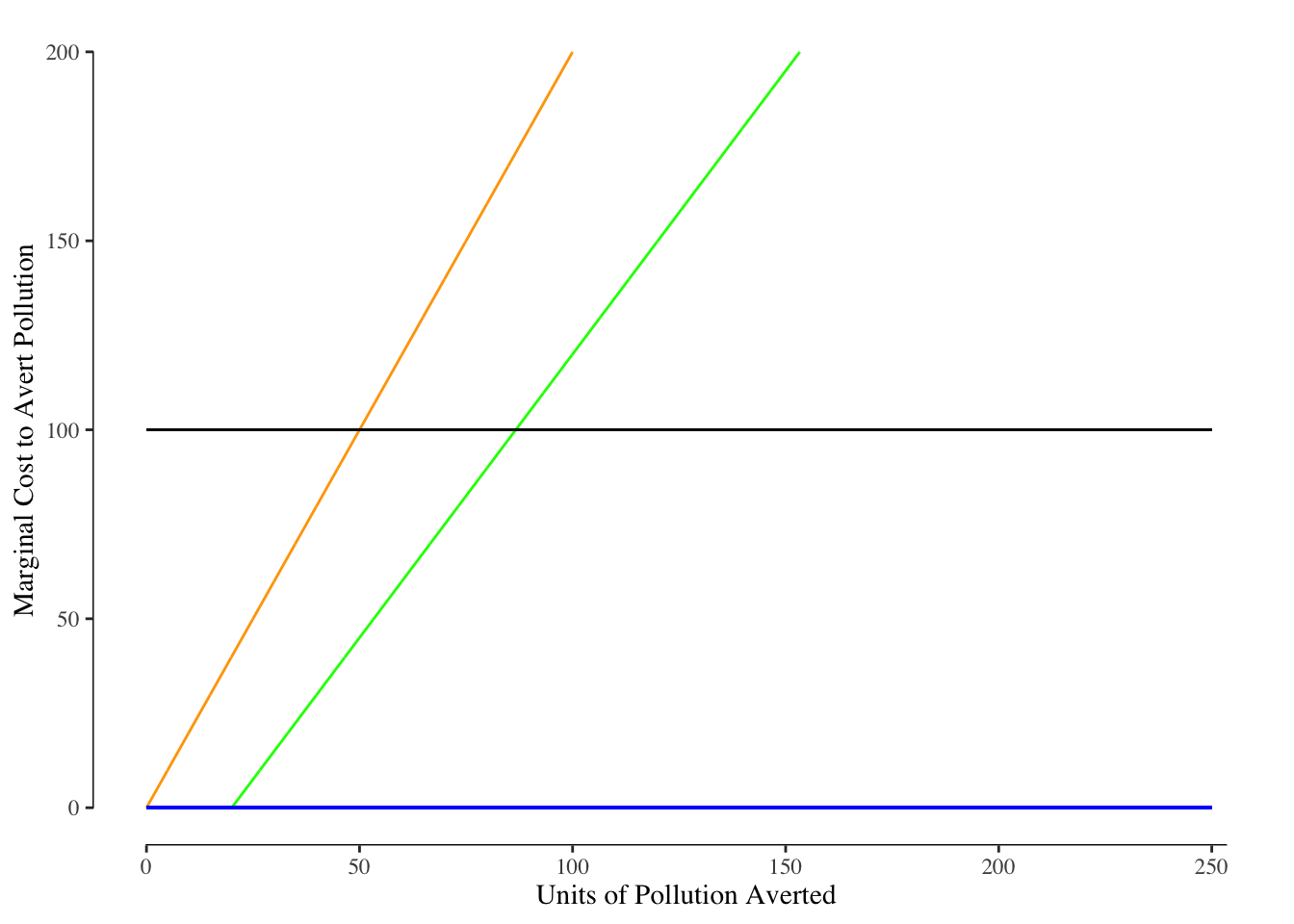
Figure 6.2: Market for Pollution Reduction. The solid blue line reflects the demand curve for both Factory A and Factory B and is constantly zero. The solid black line reflects the demand from society - in other words the marginal harm per unit of pollution. The green line is the marginal cost of reduction for Factory A while the orange line is the marginal cost of pollution reduction for Factory B.

From these two firm’s marginal costs curves, we can also draw the total marginal cost of reduction over all firms. We do this by summing horizontally over the firm’s marginal costs curves. In other words, we want to know what reduction in pollution is possible for a particular level of investment. We add this new curve to Figure 6.3.

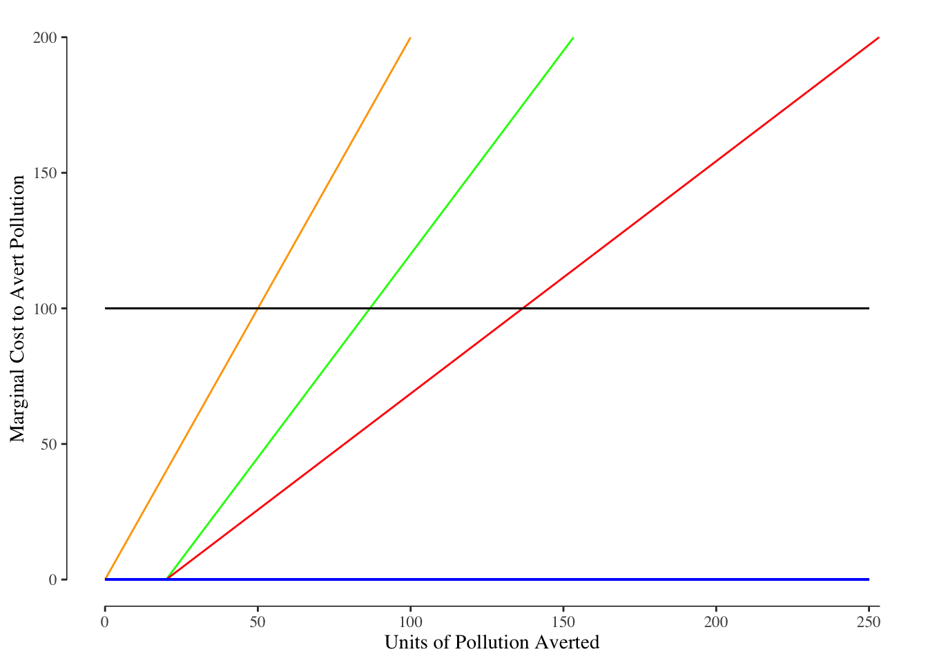
Figure 6.3: Market for Pollution Reduction. The solid blue line reflects the demand curve for both Factory A and Factory B and is constantly zero. The solid black line reflects the demand from society - in other words the marginal harm per unit of pollution. The green line is the marginal cost of reduction for Factory A while the orange line is the marginal cost of pollution reduction for Factory B. The total cost of a reduction is shown in the solid red line.

We are often interested in the total cost of the reduction, which is the sum of the costs of the reduction for the two firms. Suppose we want to reduce emissions by 75 units per factory:

\[ \text{Cost}_A = \sum_{i = 21}^{75} 1.5 i = 3,960 \\ \text{Cost}_B = \sum_{i = 0}^{75} 2 i = 5,700 \\ \text{Total Cost} = 3,960 + 5,700 = 9,660 \]

In other words, to get a 150 unit total reduction equally divided between the two firms, the total spending by the firms to reach that goal would be $9,660.

Because of the differences between the marginal cost and total cost curves for the two firms, the same reductions through price and quantity mechanisms have very different total costs.

6.3.4.1 Quantity Restrictions Only

The socially optimal reduction - the point at which the marginal cost over the two factories equals the marginal harm - is a 137 unit reduction in pollution. Let’s suppose the government takes this information and orders both factories to reduce their emissions by 67.5 units. We can draw the market for reduction and see the effects of the mandated reduction, Figure 6.4.

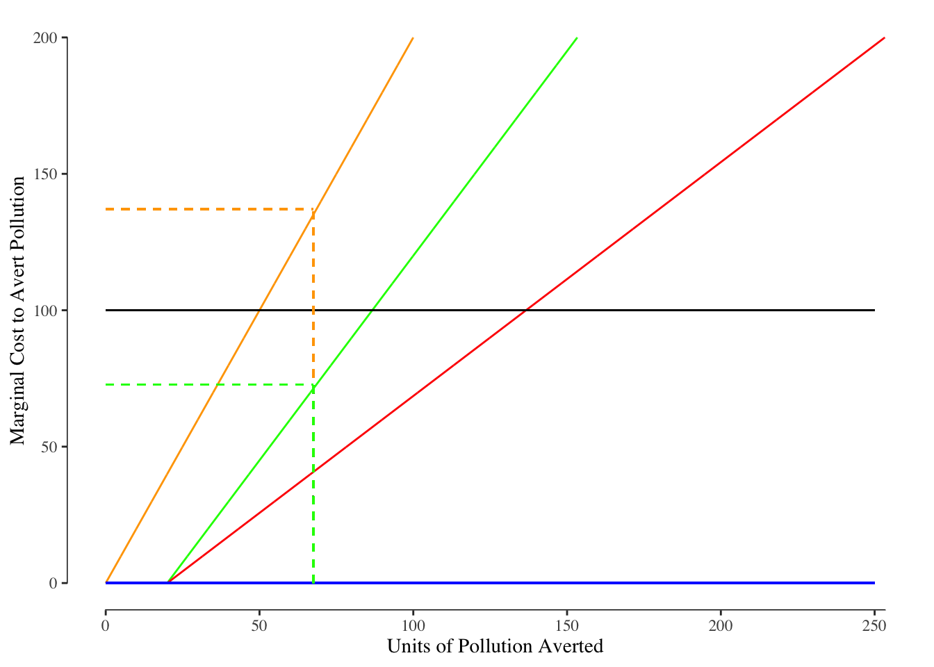
Figure 6.4: Effect of Quantity Reduction Mandate. The solid blue line reflects the demand curve for both Factory A and Factory B and is constantly zero. The solid black line reflects the demand from society - in other words the marginal harm per unit of pollution. The green line is the marginal cost of reduction for Factory A while the orange line is the marginal cost of pollution reduction for Factory B. The total cost of a reduction is shown in the solid red line. The dashed lines denote the quantity and the marginal cost assoicated with a 67.5 unit reduction in emissions.

We see both firms make the 67.5 unit reduction in emissions, but the outcome is not ideal. At a reduction of 67.5 units, the marginal cost to Factory B ($137) is well above the marginal damage caused by the pollution. The marginal cost to reduce pollution for Factory B is $37 higher than the harm caused by the pollution. Society, which includes Factory B, is worse off because the net value of the pollution reduction is negative.

Meanwhile, Factory A only has a marginal cost of $72.75 with a 67.5 unit reduction in pollution. This is below the marginal harm to society of $100. As a result, Factory A could reduce pollution by even more while still creating value for society. However, since Factory A is in compliance with the mandate to reduce pollution, Factory A has no incentive to reduce the pollution any further.

In our example, we do get the reduction of pollution that is desired by society but the cost is not minimized. Factory B is paying more than the marginal harm while Factory A is reducing less than they could while creating value for society. The total cost of this approach is²⁶

\[ \text{Cost}_A = \sum_{i = 21}^{68.5} 1.5 i = 3,255.75 \\ \text{Cost}_B = \sum_{i = 0}^{68.5} 2 i = 4,761 \\ \text{Total Cost} = 3,225.75 + 7,761 = 8,016.75 \]

6.3.4.2 Corrective Taxation Only

Alternatively, the government could impose a tax equal to the marginal damage on each unit of pollution emitted. In our example, suppose the government levies a tax of $100 on each unit of pollution. Both of our factories would response by reducing their emissions until the marginal cost of reduction was equal to $100.

To see way, consider the marginal cost function of production for each firm before the tax:

\[ \text{Marginal Cost of Production} = \text{Capital Costs} + \text{Labor Costs} \]

and when the government creates a tax it changes to:

\[ \text{Marginal Cost of Production} = \text{Capital Costs} + \text{Labor Costs} + \text{Units of Pollution Created} \cdot \text{Tax} \]

The firm cannot do anything about the value of the tax, but they can reduce the amount of pollution created by production. If it costs less than the value of the tax, the firm would prefer to reduce the pollution over paying the tax. For instance, suppose we can reduce pollution by one unit for $5 and the tax is $100. We would prefer to reduce the pollution (paying $5) than pay the tax (costing us $100). This would continue until the cost of averting the next unit of pollution costs as much as the tax. Once the tax is cheaper than the pollution reduction, we will revert to emitting the pollution and stop paying for reduction.

Turning back to our market for reduction, this means firm’s will reduce their emissions until the marginal cost of reduction equals the tax. This is shown for our two factories in Figure 6.5.

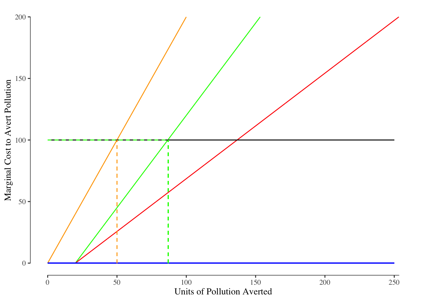
Figure 6.5: Effect of Corrective Tax. The solid blue line reflects the demand curve for both Factory A and Factory B and is constantly zero. The solid black line reflects the demand from society - in other words the marginal harm per unit of pollution. The green line is the marginal cost of reduction for Factory A while the orange line is the marginal cost of pollution reduction for Factory B. The total cost of a reduction is shown in the solid red line. The dashed lines denote the quantity and the marginal cost assoicated with a 67.5 unit reduction in emissions.

The marginal cost of reducing pollution is $100 after reducing by 87 units for Factory A and 50 units for Factory B. Note that this will cost

\[ C_A = \sum_{i = 21}^{87} = 5,427 \\ C_B = \sum_{i = 0}^{50} = 2,550 \\ \text{Total Cost} = 5,427 + 2,550 = 7,977 \]

The tax averts 137 units of pollution, the same as with a quantity restriction, but does so at a lower cost ($7,997 versus $8,016). This is because both factories engage in pollution lowering to the extent it is economical and since the tax was set to be equal to the marginal damage and the quantity cap was set based on the societal optimal quantity of reduction. The quantity cap is a crude tool that leaves “money on the table” for some firms while punishing others.

6.3.4.3 Quantity Caps with Trades

You may have heard of “cap and trade” programs to reduce emissions or other harmful externalities. These programs have been used with great success in reducing various forms of air pollution in the past. They are desirable in the sense that the quantity cap may be easier to identify than the correct tax and the ability to “trade” removes much of the excess cost creates by the quantity cap.

The way a cap and trade system works is the government issues permits to release certain quantities of pollution (e.g., they mandate a reduction in pollution) to each party. In our example of two factories, each factory would be issued half of the 137 permits. As we discussed earlier and showed in Figure 6.4, this allow would result in Factory A under reducing their emissions and Factory B over reducing compared to the net benefit to society.

The key difference here is the “and trade” concept. Let’s suppose both firms are at the point where they’ve reduced emissions by the required 68.5 units. Factory B is paying $137 while Factory A is paying $72.75. We can also think of these marginal costs as the value of the permit to emit one more unit of pollution. Factory A only values it at $72.75 while it is worth $64.25 more to Factory B. Factory A would be happy to sell the permit to Factory B for some price above $72.75 and Factory B is willing to pay up to $137 for the permit. As a result, the A will sell a permit to B, A will increase their pollution reduction efforts to 69.5 units and B will reduce their pollution reduction efforts to 67.5.

This process will repeat itself again: Factory B has a marginal cost of reduction at 67.5 units of reduction that exceeds Factory A’s marginal cost at 69.5 units of reduction. Factory A will sell to Factory B, A’s pollution reduction will increase to 70.5 units while B’s will reduce to 66.5 units. The process repeats again and again until the marginal cost of reduction for Factory A is equal to the marginal cost of reduction for Factory B. This is the point at which both firms have an equal value for the permit.

Assuming the quantity cap is correctly set, this will occur at the point where marginal costs for both firms equals the marginal damage. This will create the same level of reduction in emissions at the same cost as using a corrective tax.

6.4 Selecting Price or Quantity Approaches with Uncertainity

So far we have been pretending the government knows exactly the value of the marginal damage from an externality or knows the exact quantity that would be preferred by society. That is more than somewhat unrealistic. We’ve also been assuming that the marginal harm is constant - 10 units of pollution is equally bad for the community whether it is being added to a baseline of 5 units total or a baseline of 150 units. The harm from externalities like pollution are almost surely not a constant.

Consider \(\text{CO}_2\) being emitted and causing climate change. \(\text{CO}_2\) has a relatively long half-life (decades) and the effects of climate change are the results of the accumulated tons of \(\text{CO}_2\) emitted over the past 200 years. If society effectively erased all \(\text{CO}_2\) emissions starting tomorrow, we would be unlikely to see any short term effect in climate. Likewise, a large increase in the amount of \(\text{CO}_2\) emissions next year would not matter much either.

Think about the atmospheric carbon load like a slowly draining bathtub. The bathtub contains 150 L of water and is draining at 1 L per minute. If you scoop out a liter of water, the tub drains in 149 minutes. Likewise, if you add one liter of water, the tub drains is 151 minutes. Despite the “shock” of adding or removing the liter of water, it does not have a practically meaningful effect of the time required to drain.

Using the language we’ve developed so far, we would say the SMB of reducing \(\text{CO}_2\) is relatively flat. The marginal damage from increasing or decreasing carbon emissions requires large changes to have any meaningful impact on our outcome. We may see a SMB curve somewhat like that in Figure 6.6.

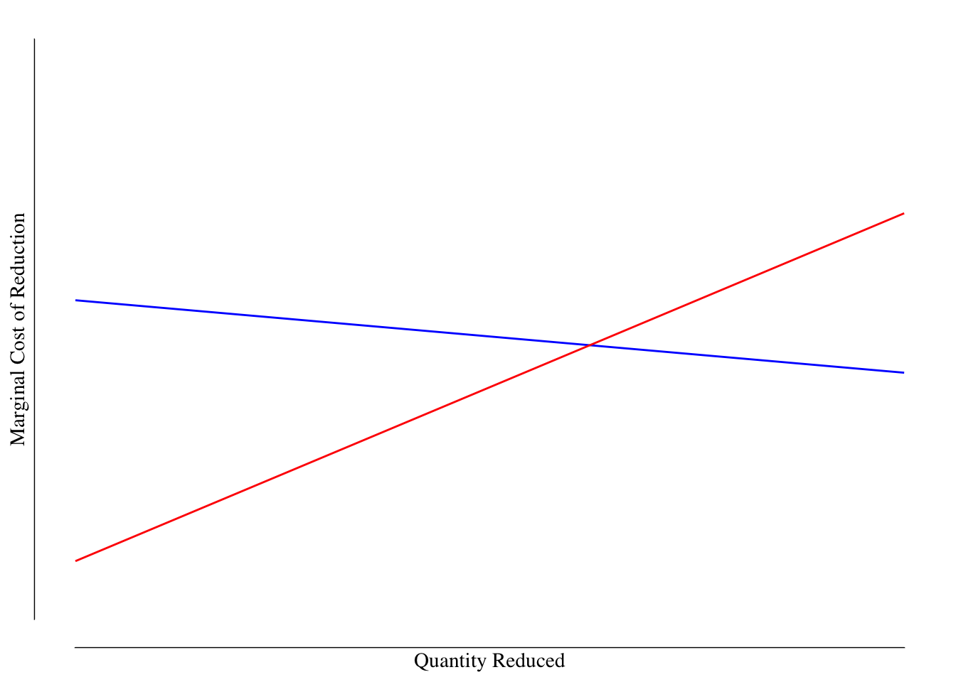
Figure 6.6: Market for $ ext{CO}_2$ Reductions. The marginal cost of reductions is shown as a solid red line and the societal marginal benefit is shown as a blue line. Because the effects of $ ext{CO}_2$ on climate relate to the cumulative burden of $ ext{CO}_2$, large changes in the quantity emitted are required for even small changes in the SMB.

The line we’ve drawn for the marginal cost is merely our best guess as to the marginal cost. Suppose we get it wrong and the true marginal cost is greater than our guess. To make this concrete, let’s suppose the red solid line denotes our expected marginal cost replacing internal combustion cars with electric cars. However, it turns out there is a new barrier to lithium production for batteries and the marginal cost of the transition increases. How would that affect our market if we use a quantity restriction or a tax?

The government could use this graph to set a quantity restriction so that the socially optimal amount of \(\text{CO}_2\) is released. They would do this at the point where the \(\text{SMB} = \text{MC}\). This would result in the optimal amount of reducing and resolves the externality. How would this affect our market? We model the change in Figure 6.7.

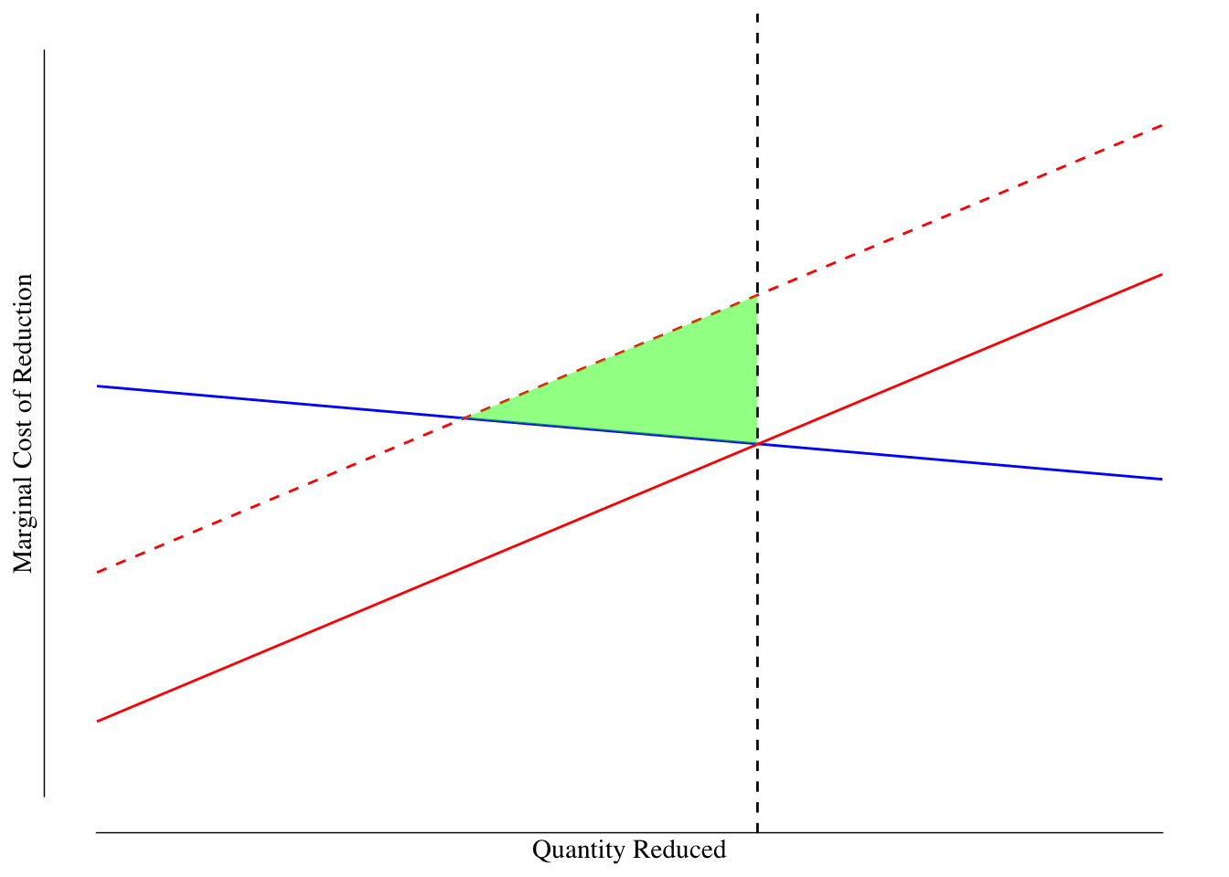
Figure 6.7: Market for $ ext{CO}_2$ Reductions With Uncertainity: Quantity Restrictions. The best estimate of the marginal cost of reductions is shown as a solid red line and the societal marginal benefit is shown as a blue line. However, the true marginal cost (dashed red line) is higher. The black line denotes the reduction required by the government based on the estimated marginal cost. The dashed black line denotes the required reduction in pollution. The deadweight loss for this policy is shown in the green shaded triangle.

Since the quantity restriction is mandated, regardless of the fact that the cost estimate was inaccurate, the firms are required to make the reductions. This creates a deadweight loss as they reduce to the point beyond which the cost of the reduction was offset by a benefit to society. This is the region between the intersection of the SMB and true marginal cost curves, above the estimated marginal cost curve, below the true marginal cost curve, and less than the required reduction.

What would happen if we instead applied a tax equal to the price at which the estimated marginal cost and SMB curves intersect? How would that affect our market? We model this in Figure @ref{fig:climate-change-3}.

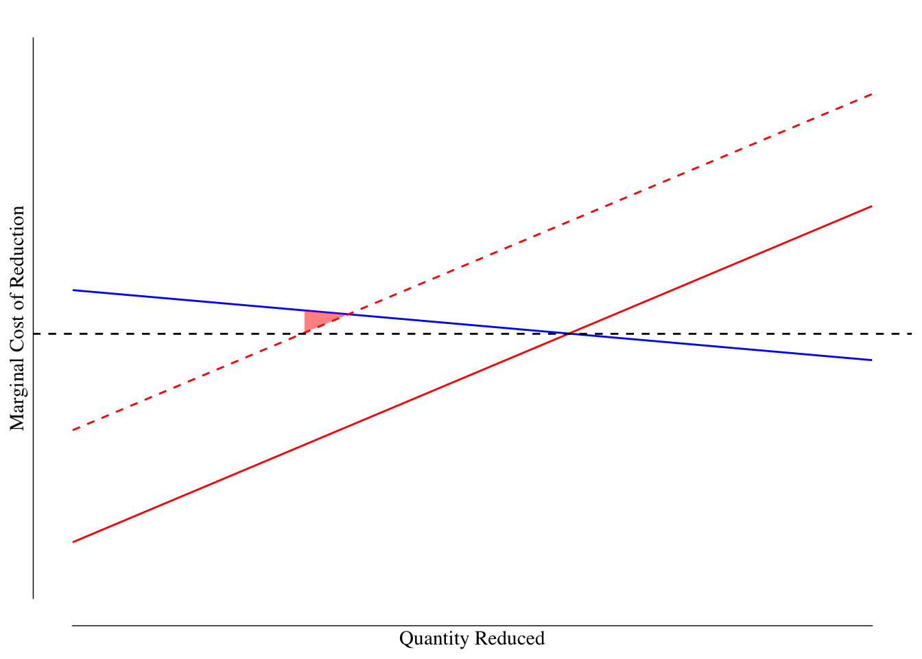
Figure 6.8: Market for $ ext{CO}_2$ Reductions With Uncertainity: Taxes. The best estimate of the marginal cost of reductions is shown as a solid red line and the societal marginal benefit is shown as a blue line. However, the true marginal cost (dashed red line) is higher. The black line denotes the reduction required by the government based on the estimated marginal cost. The dashed black line denotes the tax charged per unit of carbon. The deadweight loss for this policy is shown in the red shaded triangle.

This produces a deadweight loss because the tax was set somewhat too low when using the estimated marginal cost curve compared to the true marginal cost. As a result, there is a degree of overproduction compared to what would be ideal creating a deadweight loss, shaded in red in Figure ??.

Note the deadweight loss associated with the tax is much smaller than the deadweight loss associated with the quantity restriction. This is because the SMB curve is relatively flat. Simply allowing the producers to pay the tax if has lower efficiency loss than requiring them to meet the threshold set using the estimated marginal cost curve in the event that we underestimated the marginal costs of reduction. In this example, the deadweight loss associated with a quantity restriction is 28 times larger than the one with a corrective tax.

What if we have the opposite situation where the marginal benefit of reduction is steep like lead in drinking water? There is no safe level of lead in drinking water and it is associated with many developmental, neurological, and behavioral problems. The association is so strong that one theory for why violent crime dropped in the early 1990s was because lead was removed from gasoline increasing IQs and decreasing certain issues with lack of impulse control or learning disabilities. Unlike with carbon and climate change, in this market the SMB curve would be very steep, Figure 6.9.

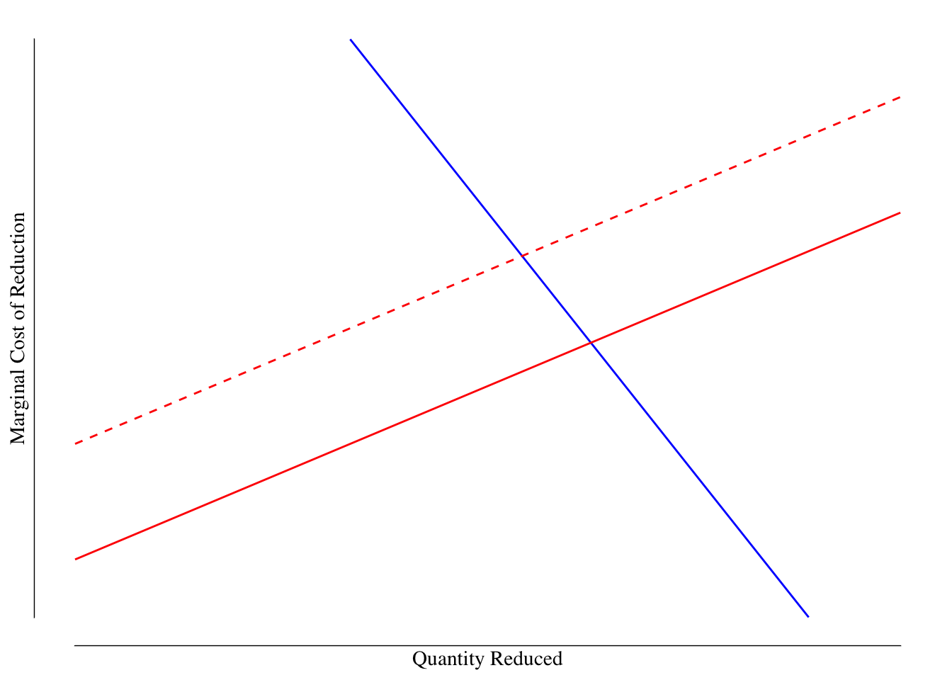
Figure 6.9: Market for Reductions in Lead in Drinking Water. The solid blue line denotes the SMB or marginal damage of lead. The red solid line is our best guess for the marginal cost of removing lead while the dashed red line is the actual marginal cost.

We have our estimated marginal cost of reduction (solid red line) and the unknown true cost, which is higher (dashed red line). How would this market respond to a quantity restriction?

We can model this in Figure 6.10. The government mandates that the lead in drinking water is reduced by a quantity equal to the quantity at the intersection of the estimated marginal cost and SMB curves. Since the true marginal cost function exceeded the estimated one, this required reducing lead at costs greater than the benefit to society. This is the area shown in green and is the deadweight loss associated with the quantity restriction.

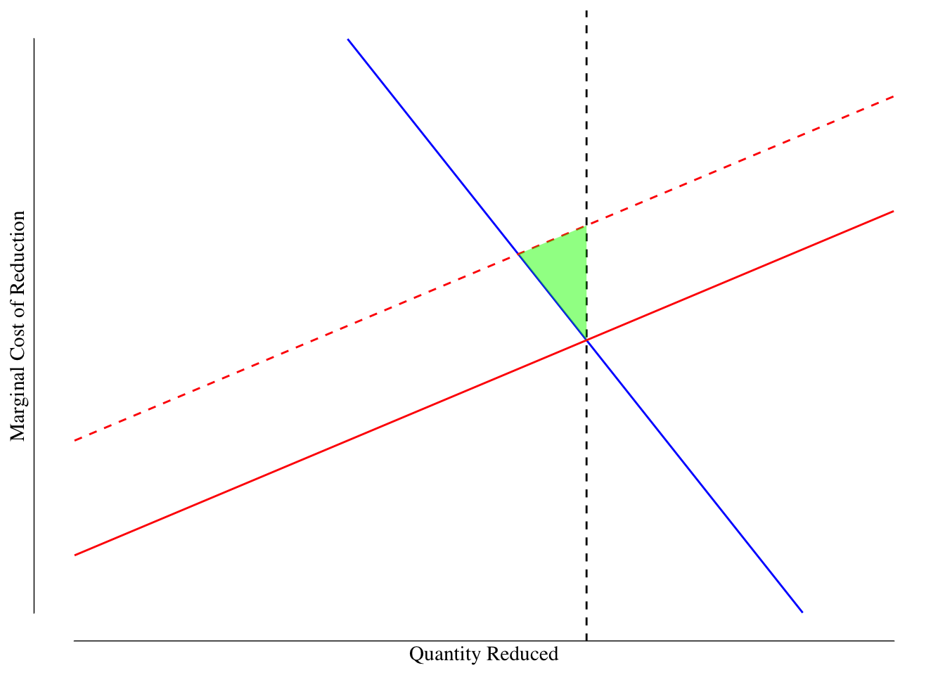
Figure 6.10: Market for Reductions in Lead in Drinking Water: Quanity Restriction. The solid blue line denotes the SMB or marginal damage of lead. The red solid line is our best guess for the marginal cost of removing lead while the dashed red line is the actual marginal cost. The dashed black line is the mandated quantity of reduction. The green shaded area is the deadweight loss.

How would taxes effect this market? The government would set the tax equal to the marginal damage given the estimated value the marginal cost curve. This is shown as the dashed black line in Figure 6.11. Since the SMB is so steep, the area between the the SMB and the true marginal cost curve is very large. This area is the deadweight loss associated with the tax when the SMB is steep and shown in red in Figure 6.11.

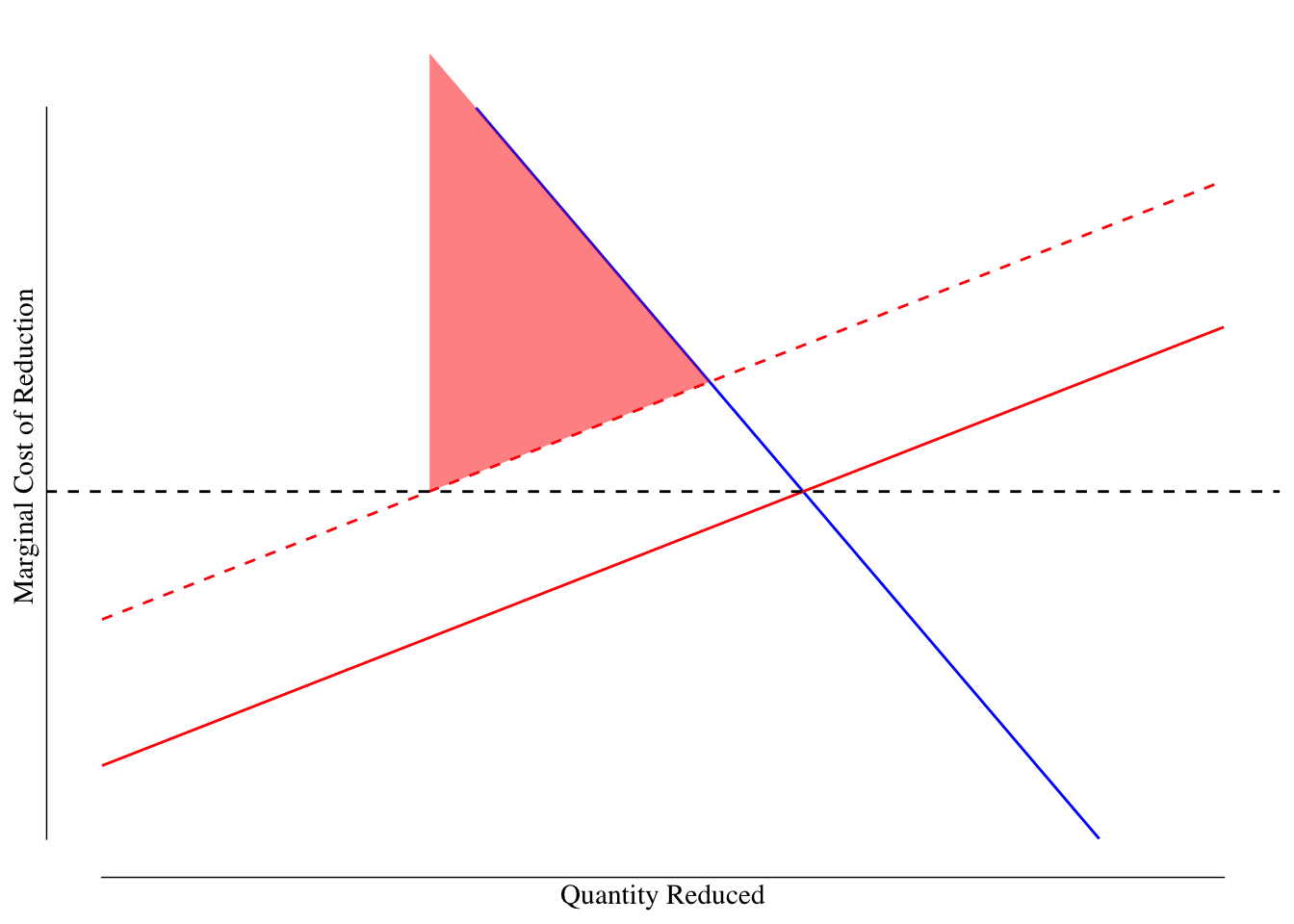
Figure 6.11: Market for Reductions in Lead in Drinking Water: Corrective Tax. The solid blue line denotes the SMB or marginal damage of lead. The red solid line is our best guess for the marginal cost of removing lead while the dashed red line is the actual marginal cost. The dashed black line is the tax. The red shaded area is the deadweight loss.

While in the case of carbon emissions, the deadweight loss associated with an quantity cap was much greater than the deadweight loss with the tax, the opposite is true in the case of lead in the drinking water. Since even small amounts of lead have large shifts in total welfare, the relationship between the two approaches flips.

These results have implications for selecting between taxes and quantity restrictions. For externalities where the SMB curve is likely very flat and there is uncertainty about the marginal cost, a tax is a “safer” bet in terms of maximizing economic efficiency. However, if keeping the quantity no higher than some threshold, as might be the case with lead or nuclear waste, it is likely that an approach based on quantity caps will be a “safer” bet to minimize the deadweight loss.

---

23. These are often in the form of tax breaks or tax credits.↩︎

24. This tax credit phases out with larger numbers of cars produced per company but the number of cars is quite large.↩︎

25. When we cover taxes, we’ll make a distinction between marginal impact of tax - the intended behavior change of the tax that actually happens - and the inframarginal impact of taxes - the tax does not change behavior as intended.↩︎

26. I’m abusing some notation in these expressions, it really should be \(1.5 \cdot 69 \cdot 0.5 + \sum_{i = 21}^{68} 1.5 i\) and likewise for Factory B since the summation expression requires whole values. But let’s roll with it anyway.↩︎